Defining capacity
Once the system and adapter parameters are defined, you add capacity to your system in the Capacity tab, one of a set of four tabs:
|
Tabs of the Projects / project_name / Systems list
|
|||
|
System
|
Adapters
|
Capacity
|
Report
|
|
Note: You can click any of the following links to learn about the other tabs in this view:
|
Select the Capacity tab, where you configure and modify pools and arrays. For device-specific details, see this topic:
“Capacity modeling the System 9152”
For limitations and restrictions on the storage systems, refer to the documentation links in
Table 28.
Tool Tip pop-up windows can appear in the upper-right corner of the view displaying functions that a model does or does not support. To close the pop-up select the “x” in the upper-right corner.
Table 28 Sample links to information: Limitations and restrictions on the storage systems*
|
“” Topic
|
Link
|
|---|---|
|
V8.5.0.x Configuration for IBM System 9500 family
|
|
|
V8.3.1.x Configuration for IBM System 9200 family
|
|
|
V8.2.1 Configuration for IBM System 9100 family
|
|
|
V8.5.0.x Configuration for IBM System 7300 family
|
|
|
V8.3.1.x Configuration for IBM System 7200 family
|
|
|
V8.6.3 -> V8.7.0.x Configuration for IBM System 5300 family
|
|
|
V8.5.1‘.x Configuration for IBM System 5200 family
|
|
|
V8.3.1.x Configuration for IBM System 5x00
|
|
|
Configuration for IBM System Storage SAN Volume Controller
▪Version 8.2.1.x
▪Version 8.5.0.x
▪Version 8.5.1.x
▪Version 8.6.3.x
|
▪
▪https://www.ibm.com/support/pages/v850x-configuration-limits-and-restrictions-ibm-system-storage-san-volume-controller
▪https://www.ibm.com/support/pages/v851x-configuration-limits-and-restrictions-ibm-system-storage-san-volume-controller
▪https://www.ibm.com/support/pages/node/7109991
|
|
Configuration for IBM Storwize V7000
▪
▪Version 8.2.1
|
▪
|
|
Configuration for IBM Storwize V5000
▪
▪Version 8.2.1
|
▪
|
|
* Limitation and Restrictions reports are regularly released. Go to
https://www.ibm.com/support/
and enter the following search string to find all available reports:
Configuration for IBM family_name Vnnnn
where,
family_name
is the name of the family you are searching for, such as
System or Storwize and
nnnn
is the family version number, such as
9200 or 5000.
|
|
Adding pools
Start by configuring a storage pool, select the
Add Pool icon, as in Figure 343. A pool or
storage pool is an allocated amount of capacity that jointly contains all of the data for a specified set of volumes. You must assign arrays to a pool to provision its desired capacity.
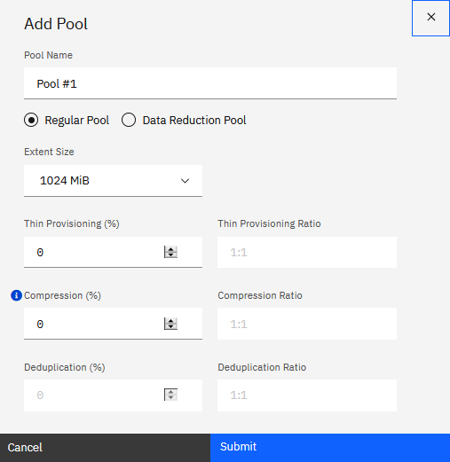
Figure 343 Defining Storage pools
Note: Compression applies only to IBM FlashCore Modules(FCM)
Note: Compression applies only to IBM FlashCore Modules(FCM)
The system supports regular pools and data reduction pools. Data Reduction Pools (DRP) are required to support deduplication and improved compression over Real-time Compression in IBM
Storage Virtualize environments. DRP also enables free capacity to be reclaimed at a finer grain of 8KB allocation blocks.
There are three software functions related to data reduction:
▪Thin provisioning
▪Compression
▪Deduplication
The three functions can be combined. For a System 9100 and the V7000 NVMe, the functions Compression and Deduplication are available only in Data Reduction Pools (DRP), while Thin
Provisioning and compression (built-in compression for FCM, software compression for other drives) can also be utilized in a Regular pool.
For the SV1, the functions Thin provisioning, Compression and Deduplication are available only in Data Reduction Pools (DRP), while only Thin Provisioning can be utilized in a Regular
pool.
|
Notes:
▪If compression is defined for devices that do not support compression, it will be ignored in the calculations.
▪As with all technical specifications, Storage Modeller dynamically answers device-level questions like this,
“What combinations of Thin provisioning, Compression, and Deduplication are valid for Regular pools? DRP pools?” Thus, you are freed from searching for such specifications. However, sometimes you need to check a specification. For search guidelines, see “Accessing technical specifications for IBM Storage Virtualize devices”. |
Extent Size: Storage pools are split into extents of the same size. A larger extent size increases the total amount of storage that the system can
manage. A smaller extent size provides more fine-grained control of storage allocation.
|
Note: Do not create DRP with an extent size that is too small. DRPs are capped at 131072 extents per IO group. A DRP with extent size 1024 MB can have a
maximum of 128 TB (13102 divided by 1024) of used capacity, within a single I/O group. A DRP with extent size 8192 MB can have a maximum of 1024 TB of used capacity, within a
single I/O group.
|
Thin Provisioning provides the ability to define logical volume sizes that are larger than the raw capacity installed on the system. That way, you can defer capacity allocation on a
storage resource until data is actually written to it.
DRP Compression: Data reduction can increase storage efficiency and performance and reduce storage costs, especially for storage.
Deduplication can be configured with thin-provisioned and compressed volumes in data reduction pools for added capacity savings.
|
Understanding data reduction rates, ratios, and savings:
To clarify the meaning of the terms
data reduction ratio, data reduction savings rate, and data reduction savings, consider a
use case where the original data size before data reduction was 100 TB, and the data size after data reduction is 40 TB.
The following values help to clarify these terms:
▪Data Reduction rate = 60%
▪Data Reduction savings rate = 60%
▪Data Reduction savings = 60 TB
▪Data Reduction ratio = original size (100 TB) divided by the size on disk after data reduction (40 TB) = 2.5:1
When you consider savings, it is easiest to use the data reduction rate.
The data reduction ratio helps in understanding how much effective data you can store on your system. So, when you have a 2.5:1 data reduction ratio, you will be able to store
250 TB of effective data capacity on 100 TB of usable capacity.
|
Once you have defined your configuration options, select
Submit. The new pool is displayed in the Capacity view, as shown in
Figure 344. In this case, the usable capacity is 133.07 TiB as a result of our
assignment of an array to the pool, as described in “Types of arrays”. Prior to addition of
an array, capacity shows as zero (0).
Modifying pools
This section describes how to modify pools and the arrays that they contain.

Figure 344 Adding and modifying storage pools and arrays
The area in
Figure 344
includes the following controls that you use to modify or delete the pools and arrays:
1. In the pools list, click the action icon (vertical ellipsis) at the right of the row for a pool:
a. Select Edit to access the
Edit pool dialog box and modify the configuration.
b. Select Virtualize to access the
Add Virtualization dialog box and make the pool virtual.
c. Select Delete to remove the pool.
2. Click the action icon (vertical ellipsis) at the right of the row for an array, and select
Edit to access the Edit Array dialog box and modify the configuration. You also have the option to select
Delete to delete the array from the system.
Types of arrays
An array is a group of physical drives. A Redundant Array of Independent Disks (RAID) is a method of configuring member drives to create high availability and high-performance systems. The
IBM Storage Virtualize systems support nondistributed and distributed array configurations.
In nondistributed arrays (known as Traditional RAID), entire drives are defined as “hot-spares.” Hot-spare drives are idle and do not process I/O for the system until a drive failure
occurs. A nondistributed array can contain 2 - 16 drives.
Distributed Arrays (DRAID) can contain 2 - 128 drives, and also contain rebuild areas that are used to maintain redundancy after a drive fails.
Distributed arrays are preferred because distributed RAID provides better performance and rebuild times. For systems that support only NVMe drives, only distributed arrays are created for
array configuration since these drives have improved performance for high-demand drives. Nondistributed RAID1 and RAID10 are also supported for non-compressing NVMe drives, but only
distributed RAID is supported for compressing drives. NVMe drives are only supported within certain models of control enclosures. Verify that your model supports NVMe drives before
completing array configuration. For systems that contain both NVMe and SAS drives, the system restricts mixing these different types of drives in the same array configuration because
members in the array must be as similar as possible to avoid performance problems and issues replacing drives.
Table 29 Details about supported drives, array types, and RAID levels
|
IBM Storage Virtualize Family
|
About drive, array type, and RAID level support
1
|
|---|---|
|
Systems
|
The Systems support IBM FlashCore Module NVMe drives, industry-standard NVMe drives, and SAS drives that are within expansion enclosures. The type and level of arrays varies,
depending on the type of drives in the I/O group. For all types of drives, distributed array level 6 is recommended. The system does not support mixing SAS drives in an array with
NVMe drives or mixing IBM FlashCore Modules in an array with industry-standard NVMe drives.
|
|
SAN Volume Controller
|
Note: The SVC Entry Storage Engine SA2 and the SVC Storage Engine SV3 cannot have internal arrays.
|
|
FlashSystem 5200, 5300, 7300, and 9500
|
The FS5200, FS5300, and FS7300 NVMe systems can use NVMe-attached drives in the control enclosures to provide significant performance improvements as compared to SAS-attached
drives. The systems also support SAS-attached drives via 24 or 96 slot expansion enclosures. The systems can also have LFF expansions.
The FS5015 and FS5045 have two control enclosure models available: a 12-bay for LFF drives and a 24-bay for SAS or spinning drives. They also support SAS drives attached with 12,
24, or 96 slot expansion enclosures.
FlashSystem 9500 supports NVMe in the control enclosures and flash drives: A9F(92 drives) or AFF(24 drives)
|
1 As with all technical specifications, Storage Modeller dynamically answers device-level questions like this,
“What drives, array types, and RAID levels are supported?”
Thus, you are freed from searching for such specifications. However, sometimes you need to check a specification. For search guidelines, see “Accessing technical specifications for IBM Storage Virtualize devices”.
“What drives, array types, and RAID levels are supported?”
Thus, you are freed from searching for such specifications. However, sometimes you need to check a specification. For search guidelines, see “Accessing technical specifications for IBM Storage Virtualize devices”.
Adding and Modifying Arrays
To add or modify an array follow these steps:
1. Add and configure an array as follows:
a. In the Capacity tab, click the caret (^) icon beside the pool name to access the
details for that pool.
b. Click the Add Array button. The Add Array dialog box is displayed.

Figure 345 Adding (or editing) an array
|
Note: The Edit Array dialog box presents the same options as Add Array. Exception: You click a
Save button (not Submit) to save edits to an array.
|
c. Assign the I/O group by selecting the drop-down icon, and selecting the I/O group to use.
By default, a system is configured with only one I/O group. If you have configured a system with multiple I/O groups, then you can select by array set definition into which I/O group the
drives should be placed.
d. Select the Effective Capacity or
Number of Drives radio button, according to these guidelines:
– Effective Capacity: Use this option to specify the requested
effective capacity number of drives. (Refer to
“General storage terminology used in Storage Modeller”
for the definition of
effective capacity.)
With this option, Storage Modeller takes these actions:
With this option, Storage Modeller takes these actions:
• Dynamically configures the array to match the
Effective Capacity value that you enter.
• Assigns the Automatic option in the
Rebuild Areas field. This option implements the IBM best practice (see
“Benefits of the Automatic option”). You can always override this selection and enter a
specific number for Rebuild Areas.
– Number of Drives: Use this option specify an exact number of
drives for your array. By default, Storage Modeller sets the Rebuild Areas field to Automatic, but you are free to modify this setting. Some additional factors:
• For traditional non-distributed arrays:
The number of drives that you specify does not include spare drives. It includes only parity or mirror drives.
• For distributed arrays: The number of drives that you
specify includes the distributed spare blocks. The spares are not actual drives, but empty blocks on all drives in the array.
e. As needed, adjust the values for drive technology and type, RAID type, rebuild areas, target grouping, maximum
array width, and strip size.
f. Click Submit. The new array is visible at the bottom of the array section
of the Pools view.
|
Troubleshooting tip:
If the array is not added/updated, analyze error messages that might be displayed. For example, invalid values trigger display of a message like this:
Example 1 ‘Invalid value’ error message when you attempt to add an array
Maximum of 24 NVMe drives per control enclosure.
SCM + NVMe drives cannot exceed 24 drives per control enclosure.
In the
Add Array dialog box, fix the value that is in error (see, “Resolving array configuration errors”
as needed), then again click
Submit.
|
After the array is added, the Pools view is displayed again with your modifications to Usable and Effective capacity. (For example, see the display in
Figure 344 on page 391.)
See
“Capacity calculation with IBM FlashCore Modules(FCM)”
for details on how Storage Modeller calculates and displays the raw and effective capacity with self-compressing FCM drives.
2. Modify or delete existing arrays as follows:
a. Expand the row of the pool whose array you want to modify.
b. Click on the “action icon” for the array to access the operation you want to perform:
Edit or Delete.
Tips regarding selected fields in the Add Array dialog box:
▪Strip Size: Strip size multiplied by the number of disks in the array determines the strip size value. Strip size can be any power of 2, from 4 KB
to 128 MB. When defining a striped logical volume, at least two physical drives are required. The size of the logical volume in partitions must be an integral multiple of the number of
disk drives used. (Regarding strip and stripe, see
“General storage terminology used in Storage Modeller”.)
▪Target Grouping: Select the number of drives, adding parity drives (1 parity drive (P) in DRAID5 or 2 Parity drives (P + Q) for DRAID-6.
▪Drive Types: A message label will alert you if you select a drive type that has been withdrawn from Marketing.
▪Max Array Width:
You can specify the upper limit for array width. If your setting exceeds what is physically possible (for example, higher than the number of drives), Storage Modeller saves this value as
part of the array configuration, but ignores it in its calculations.
▪As with all technical specifications, Storage Modeller dynamically displays the available options for array configuration. Thus, you are freed from searching for such specifications.
However, you might want to validate specifications. For search guidelines, see
“Accessing technical specifications for IBM Storage Virtualize devices”.
Automatic settings for Rebuild Areas
A typical array includes rebuild areas that help with maintenance of redundancy after a drive fails. For most drive types, you can customize the allocations of rebuild areas. You can
select
Automatic, or you can specify a specific number of rebuild areas. The Automatic option implements the IBM best
practice for allocation of rebuild areas, as described in
“Benefits of the Automatic option”.
When Storage Modeller applies an
Automatic setting, you can always override it to match your system requirements or local best-practice requirements. For example, some customers
request over-allocation in a model to anticipate future expansion of capacity.
|
Note: For some types of RAID, the Rebuild Areas field is not available (is grayed out).
|
Due to the
“Benefits of the Automatic option”, the
Rebuild Areas field is restored to the default setting of Automatic when you change the
Add Array or Edit Array options that are listed here. (You can always modify the restored setting of
Automatic.)
▪Drive Technology
▪Enclosure Type
▪Drive Type
▪Change the radio-button selection from Effective Capacity to Number of Drives, and vice versa.
▪I/O Group (The restore happens only if this change affects one of the other fields in this list.)
Benefits of the Automatic option
The Automatic option in Storage Modeller applies the following IBM best practice for rebuild areas:
One area for every set of 32 or fewer drives.
This option brings these benefits:
▪Makes your system design more flexible and portable across your design portfolio in Storage Modeller.
▪Optimizes your rebuild-area allocations, as described in
“Tracking Rebuild Areas in the Report tab”.
Tracking Rebuild Areas in the Report tab
Storage Modeller summarizes your array configurations in the Report tab for each system. When you access the
Configuration worksheet in the Report tab, you see the Rebuild Areas columns by scrolling to the right
side of the spreadsheet.
Figure 346 on page 396
shows the following report features when you have selected the
Automatic option:
▪The Rebuild Areas data is prefixed with the Automatic label. These results are visible in both the upper
Array Summary section and the lower Array Details section.
▪There are 129 drives in this sample array configuration. The Automatic option always applies the best practice standard of 1 rebuild area for every
32 drives. Here, we achieve the best practice standard by allocating 2 rebuild areas to the drive set of 33. The other drive sets have 32 drives, so one rebuild area is sufficient.
|
Note: If we had entered an integer value for Rebuild Area, the only possible single setting would be
2, which results in a total allocation of 8 rebuild areas. In contrast, by choosing the
Automatic option, we get an optimized allocation of 5 rebuild areas.
|

Figure 346 Configuration report showing Automatic calculations for Rebuild Areas