Exploring measurement error mitigation with the Mthree Qiskit extension

Quantum computers have the potential to solve valuable problems at scales inaccessible to classical computation, but they are susceptible to errors caused by noise in their environments. To tackle useful problems with quantum computation, we must deploy error handling methods that compensate for those errors. Eventually, researchers hope to achieve quantum error correction, a future capability that will allow quantum computers to correct errors as they appear during computations. Until practical error correction becomes a reality, we rely on simpler error handling methods like quantum error mitigation.

Quantum error mitigation refers to post-processing techniques that allow researchers to counteract the effects of noise once computations are complete. Until error correction becomes a reality, near-term quantum experiments will rely heavily on error mitigation. Error mitigation played a pivotal role in the 2023 IBM Quantum “utility” experiment, and there's also good reason to believe error mitigation will be important for reducing overhead requirements to enable quantum error correction and the truly large-scale quantum applications of the future.

But to realize the full potential of quantum error mitigation, we must continuously develop tools that allow researchers to apply the latest error mitigation techniques in their experiments. More specifically, we must deliver well-tested, performant software that helps to accelerate research in the field. By experimenting with these tools, quantum computational scientists will gain important insights that will help them use error mitigation more effectively.

In this blog post, we’ll take an in-depth look at one such tool, currently available in the qiskit-extension module, Qiskit-Extensions/mthree. This software package, colloquially referred to as Mthree or M3, implements the matrix-free measurement mitigation (M3) method, which is designed for scalable measurement error mitigation on quantum computing platforms.

What are measurement errors?

M3 is a quantum error mitigation package that focuses specifically on what we call “measurement errors.” While there are many different types of errors present in current and near-term quantum computers, measurement errors are among the most common. The measurements we perform to collect information from the qubits in our circuits have the largest error rates of any single instruction we can give a quantum computer. Therefore, measurement errors have a substantial impact on near-term, short-depth circuits. Fortunately, the effect of measurement errors is well described by a simple linear system as follows:

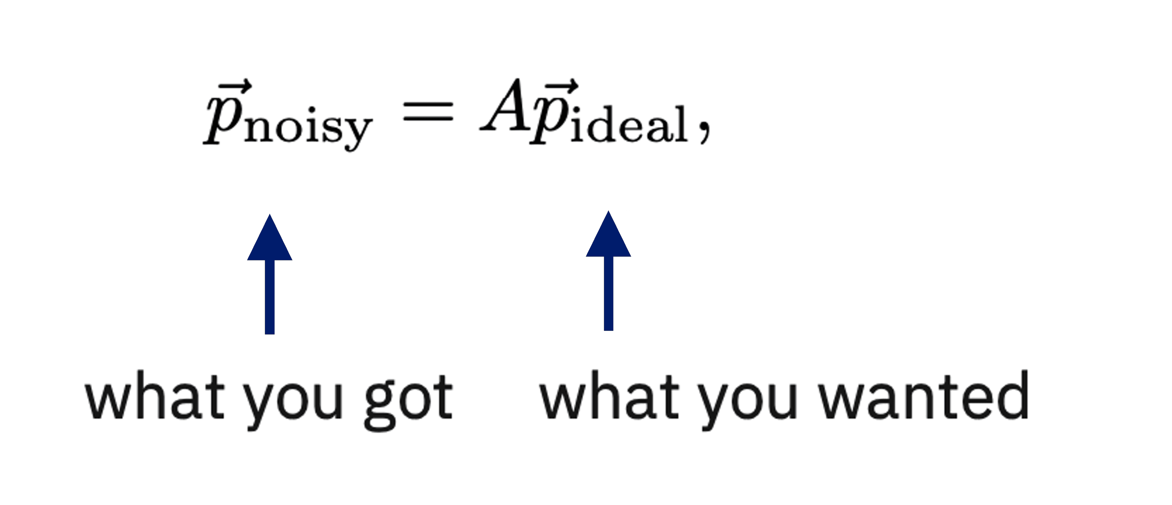
where $\overrightarrow{p}$_{$\mathit{noisy}$} and $\overrightarrow{p}$_{$\mathit{ideal}$} represent the output probability vector of the measured bit strings with measurement noise and without measurement noise, respectively. Here, $\mathit{A}$ is the $\mathrm{2}$^$\mathit{n}$$\mathrm{×2}$^$\mathit{n}$ “Assignment” matrix (where $\mathit{n}$ is the number of qubits) that probabilistically maps a given ideal measurement outcome to the noisy outcome we actually observe.

Naively, we can mitigate the measurement errors by multiplying the inverse of the assignment matrix, $\mathit{A}$^{$\mathrm{-1}$}, with the output probability vector of the measured bit strings, $\overrightarrow{p}$_{$\mathit{ideal}$} . In this case, we can construct $\mathit{A}$ by executing circuits for the $\mathrm{2}$^$\mathit{n}$ basis states and measuring them in the computational basis. However, as you might imagine, this approach is not practical for large numbers of qubits, since the number of circuits to run and the dimensions of $\mathit{A}$ and $\overrightarrow{p}$ grow exponentially with $\mathit{n}$.

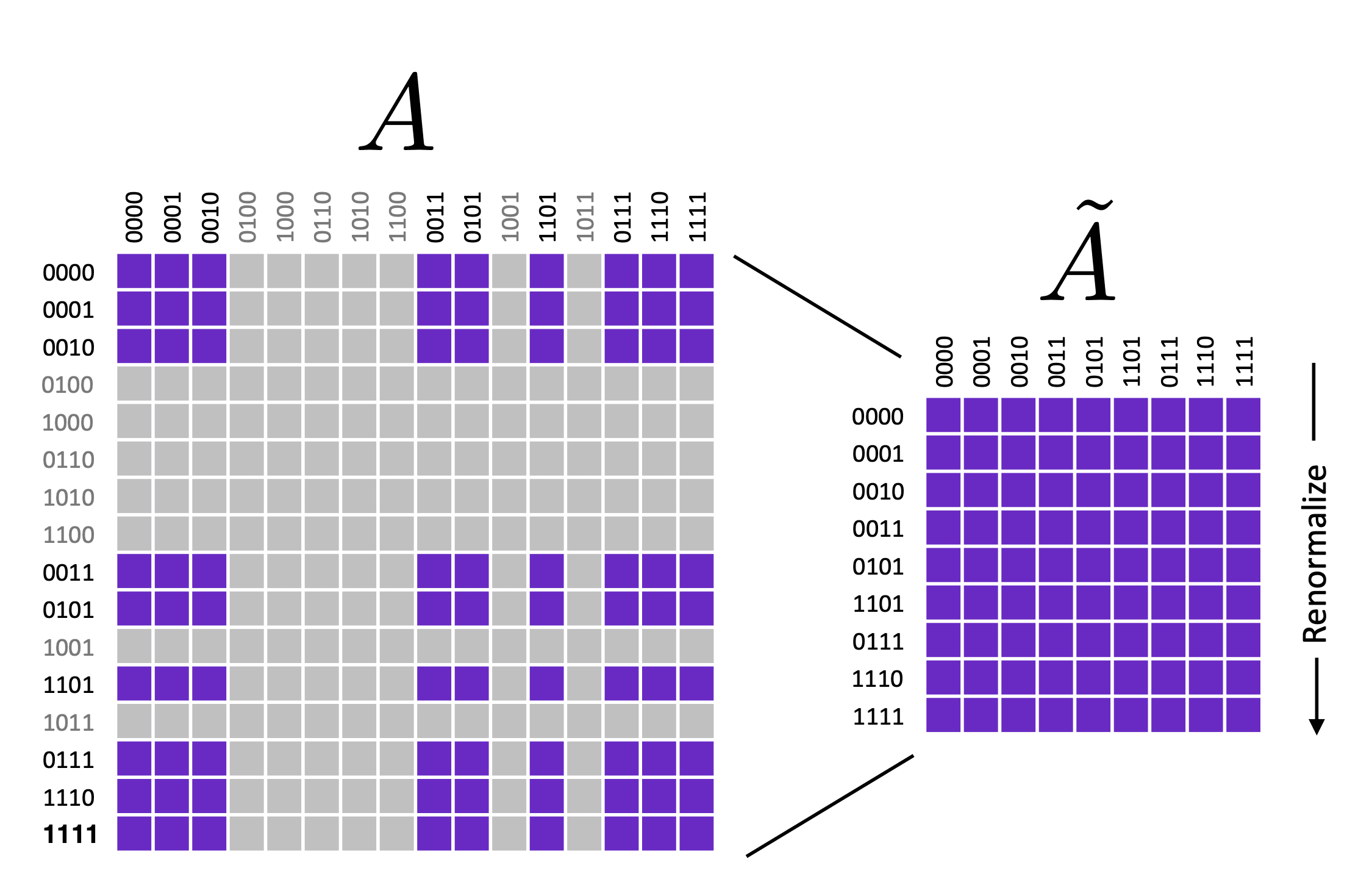
One idea for alleviating these resource requirements is to approximate $\mathit{A}$ by performing a tensor product of the $\mathrm{2×2}$ assignment matrix of each qubit, assuming there is no correlated error. In this case, we need $\mathrm{2×}\mathit{n}$ basis state circuits, where we prepare each circuit pair in the basis states of an individual qubit, 0 and 1, and then measure them. Although we can use tensor product approximation to reduce the required number of calibration circuits to be linear in the number of measured qubits, the dimension of the assignment matrix remains exponential, $\mathrm{2}$^$\mathit{n}$$\mathrm{×2}$^$\mathit{n}$. This is one of the main issues that most measurement error mitigation methods face.

How M3 tackles quantum measurement errors

M3 can help us sort out this problem. If measurement errors are small — on the order of a percent or so — and circuits are sampled sufficiently, M3 can take advantage of the fact that the noisy outcome bit strings actually contain all the ideal bit strings as a subset; the signal is hidden in the noise.

Instead of working with the full $\mathrm{2}$^$\mathit{n}$$\mathrm{×2}$^$\mathit{n}$ $\mathit{A}$ matrix, we can perform error mitigation in a reduced $\mathit{k}\mathrm{×}\mathit{k}$ subspace defined by the $\mathit{k}$ unique bit-strings in the noisy output. With $\mathit{k}$ being at most equal to the number of samples taken (number of shots), $\mathit{k}$ can be much smaller than $\mathrm{2}$^$\mathit{n}$, especially for a large $\mathit{n}$.

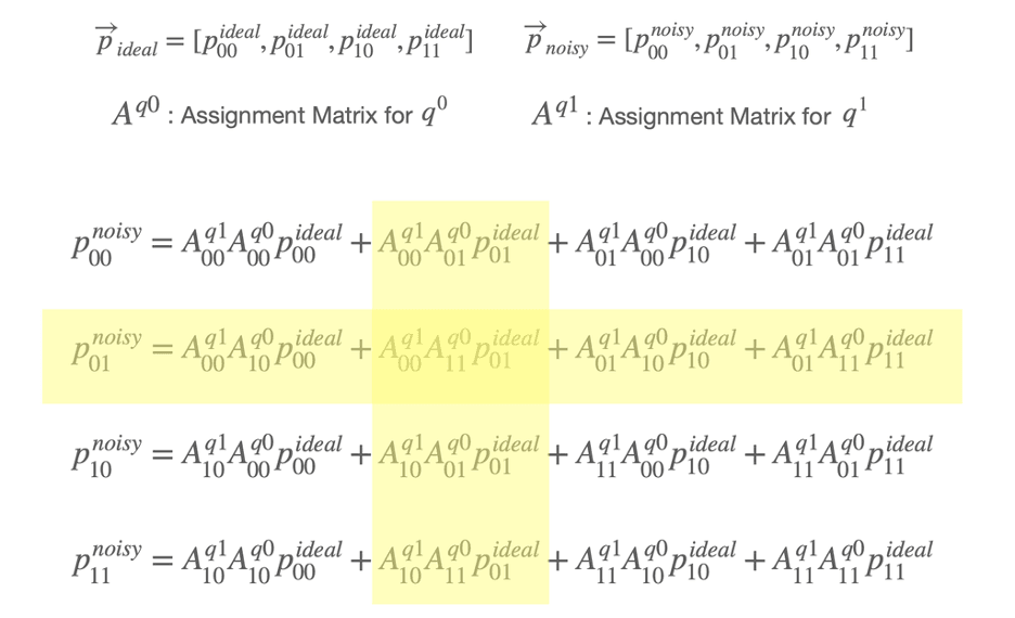
To understand this idea in detail, let’s consider a simple two-qubit example.

Suppose that, out of four possible bit strings, we obtain three bit strings — 0 (00), 2 (10), and 3 (11) with some probabilities denoted by $\mathit{p}$_{$\mathit{ij}$}^{$\mathit{noisy}$}, as shown in the figure below. With enough shots and an error rate of only a few percent, we can ignore the terms in the shaded yellow region. This reduces the $\mathit{A}$ matrix dimension down to $\mathrm{3×3}$ from $\mathrm{2}$^$\mathrm{2}$$\mathrm{×2}$^$\mathrm{2}$. This truncation can be huge when we’re working with a large number of qubits, and therefore reduces the matrix size of $\mathit{A}$ dramatically.

Of course, there are also cases where the number of output bit strings is so high that even the reduced assignment matrix, $\tilde{A}$, could be larger than the available memory. In these cases, M3 solves the systems of linear equation iteratively, without constructing any matrix.

Iterative methods are usually slow. However, M3 takes advantage of the fact that $\tilde{A}$ is diagonal dominant thanks to the small size of the measurement error. Applying a preconditioning technique and starting the iterations at $\overrightarrow{p}$_{$\mathit{noisy}$} results in rapid convergence in just a few iterations using orders of magnitude less memory.

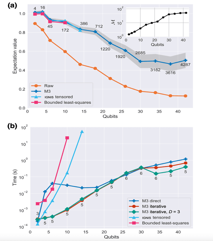
Below is a figure from our paper showing M3 performance compared to other mitigation methods in terms of accuracy and speed. Here, we use a GHZ circuit running on the IBM Quantum Brooklyn system and varying number of qubits up to 42.

At 42 qubits, M3 iteratively mitigates the errors in 1.2 seconds at most and uses about 1 megabyte of memory. This is impressive given that the size of the memory required to store sparse full $\mathit{A}$ matrix for this case is about 580 PiB. That’s 120x more memory than that of Fugaku, widely regarded as one of the fastest supercomputers in the world.

However, being able to mitigate the impact of measurement error efficiently, even at large scales, doesn’t come for free. Applying M3 will improve the accuracy of your results, but it also increases the uncertainty.

We can compensate for this by taking more samplings. The size of the sampling overhead is bounded by a multiplicative factor, $\mathit{M}$, which we can estimate using the one-norm of the inverse of the reduced assignment matrix as $\mathit{M}$ $\mathrm{=}$ $\lVert$ $\tilde{A}$^{$\mathrm{-1}$} $\rVert$^$\mathrm{2}$ . This indicates the number of additional shots M3 needs to take to make up for the unavoidable loss of precision.

M3 in action

Now that we have a good theoretical understanding of the method that powers M3, let’s wrap things up with a simple example that will show you how to actually use it. To execute the codes shown below, you’ll need to install M3 by running the command found on this page.

The following code constructs Bernstein-Vazirani (BV) algorithm circuits and executes them on a hypothetical system we call FakeSherbrooke. There are a total of eight circuits and the number of qubits in each circuit grows by one starting from two. All the BV circuits here are designed to produce $\mathit{m}$-bit strings of 1, where $\mathit{m}$ is the number of qubits in the circuit. So, for example, a circuit with three qubits should generate 111 when executed.

Results we obtain from the FakeSherbrooke backend are impacted by various types of noise including measurement noise. The effects of this noise increase with the size of the circuit as shown in the success probability figure below (labeled as “Raw”).

We implement M3 on the noisy impacted results by following three steps. First, we find the physical qubits that the virtual qubits map to. Next, we perform calibration on the physical qubits to obtain their measurement noise profile. And finally, we apply the correction on the counts achieved from the circuit run. We can see how success probability improves in comparison to the raw results in the same figure below (labeled as “Mitigated”).

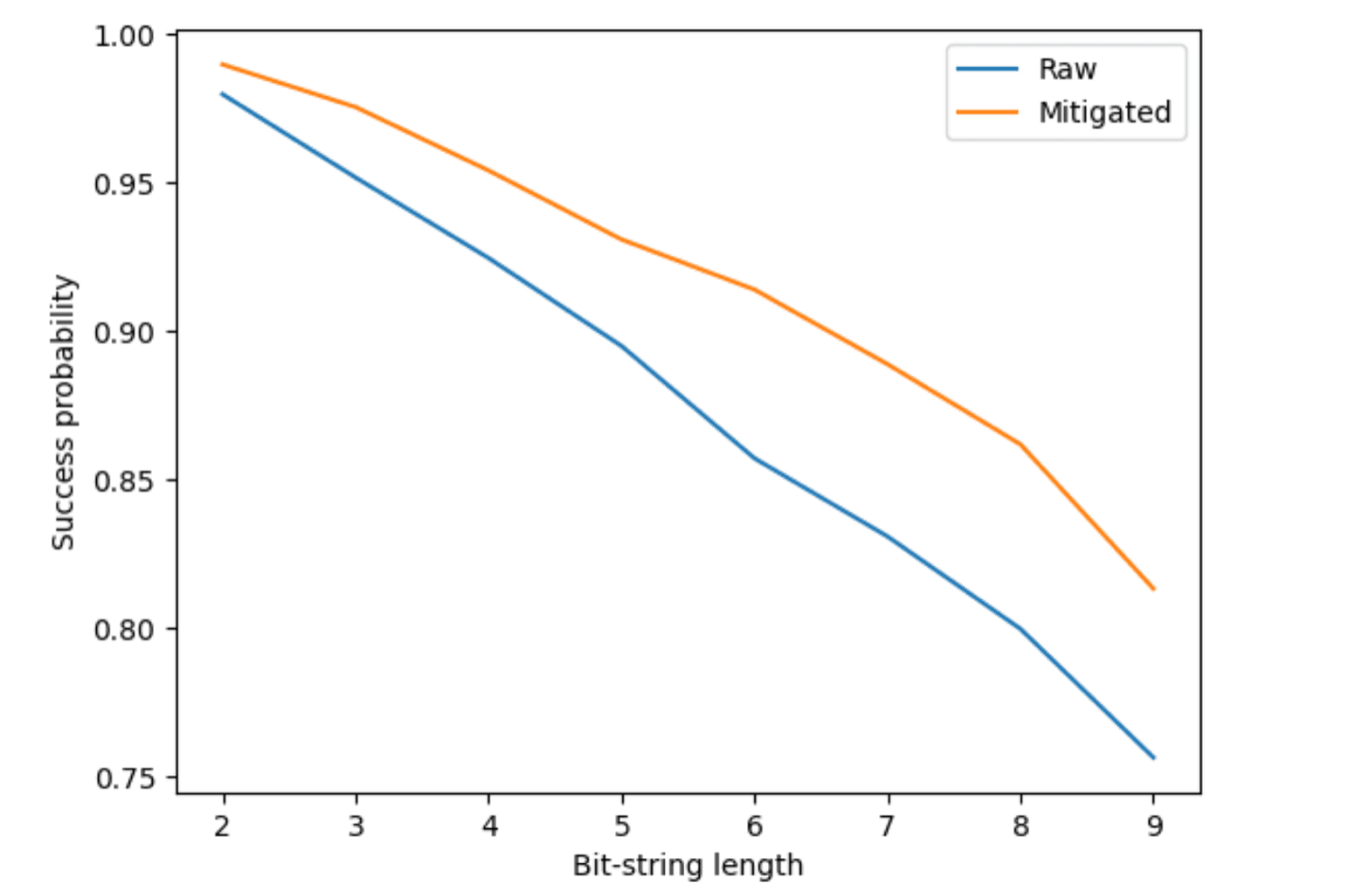
Making M3 even better

The Bernstein-Vazirani algorithm can also be realized a lot more efficiently by utilizing mid-circuit measurements. And by combining mid-circuit measurements with M3 measurement error mitigation together, we can achieve an enormous improvement in the success probability, as illustrated here.

Of course, as with any piece of code, there are still areas for improvement. One of our chief research priorities right now is finding ways to remove bottlenecks. At present, the main bottleneck in M3 is in the renormalization step for constructing $\tilde{A}$. This is an embarrassingly parallel task involving simple floating-point arithmetic. This is an ideal use case for Graphics Processing Units (GPUs), where the many parallel threads can offer a dramatic speed up.

We hope other members of the quantum community will find M3 useful, and we invite everyone to contribute to our open-source project. Together, we can push the limits of quantum error mitigation methods, and discover the true utility — and one day, even the advantage — of quantum computation.