Utility-scale dynamic circuits now available for all users

Dynamic circuits are a powerful capability that allow us to leverage real-time classical logic within the runtime of quantum circuits, making it possible to explore complex problems and diverse use cases that may be inaccessible to traditional “static” circuits with comparable resources. Now, we’re rolling out a major update that brings this capability to the utility scale, and we’re making it available to all our users—including you!

Read our documentation to get started with new utility-scale dynamic circuits.

Dynamic circuits first arrived in Qiskit Runtime in 2022, and since then, IBM® and its partners have delivered many promising demonstrations of just how potent they can be. They’ve enabled new progress in quantum error correction, novel approaches to long-range qubit entanglement, and promising experiments involving complex state preparation protocols. However, in most cases, demonstrations like these were impossible to scale beyond a certain point with the capabilities available to everyday users. Now, we have removed these barriers, and we’re empowering every Qiskit Runtime user to explore the full potential of dynamic circuits at utility scale.

Utility-scale dynamic circuits are still a work in progress, and we plan to enhance them with additional features and performance improvements over time. However, they already represent a tremendous advance in terms of the problems and applications we can explore with today’s quantum computers.

The new dynamic circuits deliver significant performance improvements over their predecessors, with one simulation experiment showing a 28% reduction in two-qubit gates for each Trotter step—a small increment of simulation time—and up to a 24% improvement in performance over corresponding unitary circuits.”

These improvements were powered by significant reductions in the duration of classical operations, and by new features such as parallel execution of conditional operations—more on those later. This means you can use the new dynamic circuits to do things that were impossible a few months ago, and we expect them to get even better as we integrate feedback from the community.

We hope you’ll start experimenting with this capability right away, so you’ll be ready to take full advantage of utility-scale dynamic circuits as they mature. Below, we detail the major changes the new implementation of dynamic circuits introduces. Before we do that, let’s run through a quick refresher:

What are dynamic circuits?

Traditional quantum circuits, or static circuits, take qubits set in some initial quantum state and apply a fixed sequence of quantum logic gates. When quantum logic operations are complete, we apply measurements and get a result.

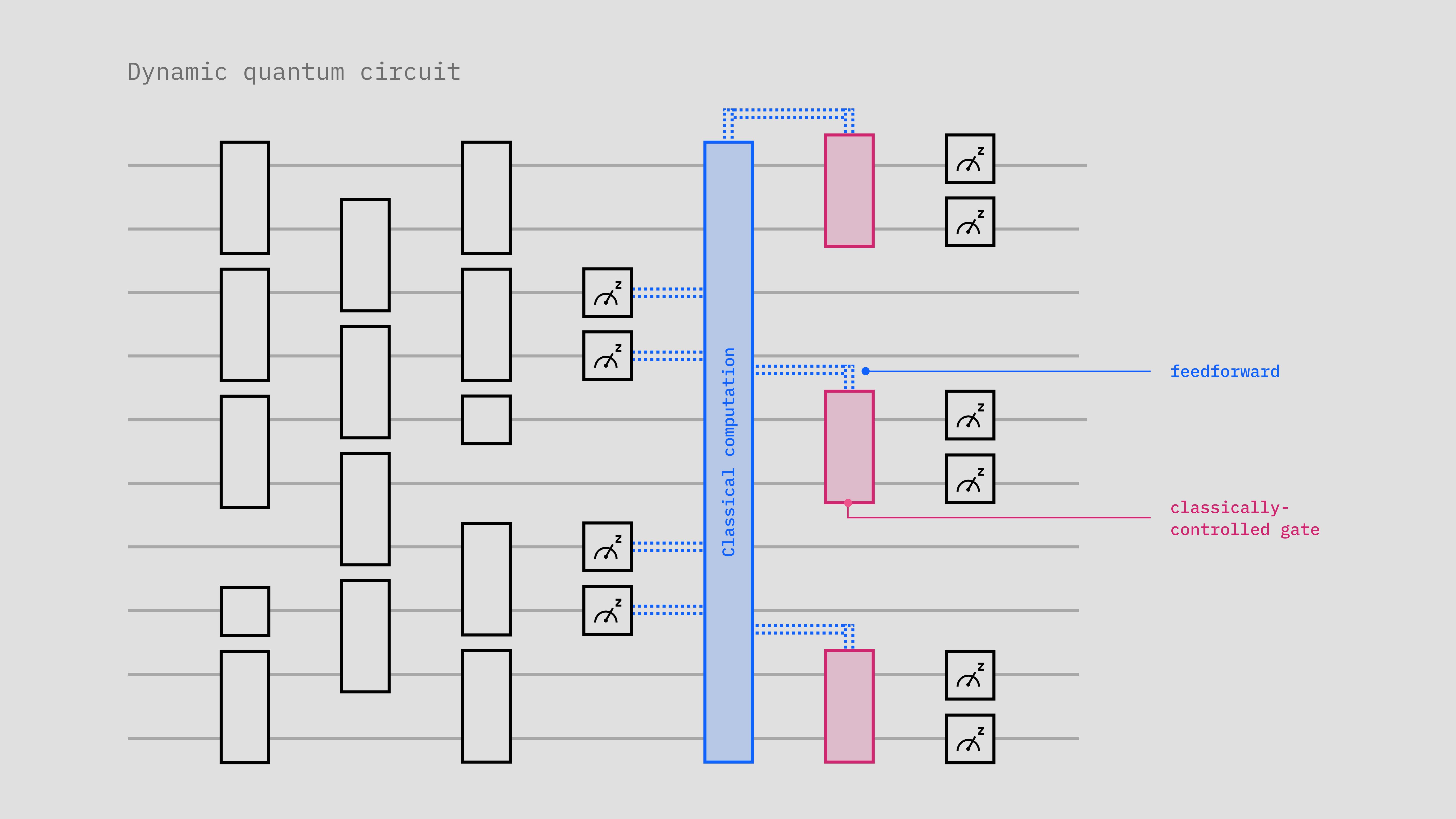
Dynamic circuits are different because of how they leverage mid-circuit measurements, which we use to measure the value of a qubit before a circuit execution is complete. Unlike static circuits, dynamic circuits use classical compute and conditional logic to decide which quantum operations we should perform in the next part of the circuit based on the outcomes of the mid-circuit measurements. This is known as classical feedforward.

With the ability to execute conditional logic operations in parallel across disjoint sets of qubits, you can implement many complex quantum protocols in constant or shallow circuit depth. This means the number of time steps required to execute all quantum operations in a circuit either remains constant or scales only modestly as we add more qubits to the system.

The new dynamic circuits won’t always outperform equivalent static circuits in terms of total runtime, particularly at smaller scales. Classical operations like mid-circuit measurement and feedforward are relatively slow compared to quantum gate operations, so they add significant runtime overhead.

Still, in cases where favorable scaling exists, dynamic circuits can deliver faster runtimes for larger problems involving more qubits. We already have multiple examples of circuits that demonstrate this scaling advantage, and we’re introducing substantial speedups to our mid-circuit measurements and classical feedforward to improve them further. This makes them a promising tool for exploring utility-scale problems that are candidates for near-term advantage

What’s new in the updated dynamic circuits

Dynamic circuits have enormous potential to extend the reach of quantum computational methods, but their original 2022 implementation in Qiskit Runtime had several limitations. They were based on an execution model that required a circuit’s control flow—i.e., its ability to execute quantum operations based on the outcomes of mid-circuit measurements—to be global. This meant that conditional operations affecting different parts of the circuit had to be executed sequentially.

In some cases, users could cleverly leverage switch statements to approximate a level of parallelism, but this method couldn’t scale beyond 10 qubits. Even at that small scale, this configuration gave users no insight into the final timing of the circuit. That’s why we built the new dynamic circuits implementation from scratch, setting ambitious goals for performance and behavior.

In terms of performance, utility-scale dynamic circuits deliver big improvements over their predecessors. Mid-circuit measurements are enhanced with a new MidCircuitMeasure instruction now capturing the results of qubit measurement nearly a full microsecond (940 ns) faster than the previous implementation, delivering a 65% improvement in duration when used for dynamic circuits. Feedforward latency is also down to around ~600ns, comparable with industry standards.

Beyond performance improvements, we introduced a new sequence translator—the tool that takes ISA circuits as input and generates the final payload that will run on the target hardware—and outfitted it with capabilities that return actionable information from the runtime to give you a better sense of how your circuits will run on the QPU. This has driven a 20x improvement in payload generation time.

We’ve also built powerful new features to overcome many of the limitations described above. These include:

Parallel execution of conditional operations

The new dynamic circuits infrastructure that can detect independent sets of conditional operations, and execute those operations in parallel. Here, “independence” means the conditional operations act on a particular group of qubits and do not interfere with any others.

Previously, dynamic circuits executed conditional operations one after the other, a process so slow that qubits would decohere before the system could finish running through all your if statements. Parallel execution of independent conditional branches brings significant improvements in circuit depth and execution time, lowering noise and improving the fidelity of results.

These performance enhancements mean we can now scale to full device utilization, leveraging all 100+ qubits of a utility-scale quantum computer.

Support for stretch duration in delay instructions

Classical feedforward makes dynamic circuits powerful, but it also makes circuit scheduling complex. Classical operations must occur in real time and can vary immensely depending on the operation complexity and target hardware specifications.

Qiskit has no mechanism for reliably modeling the execution time of the data movement or classical operations involved in feedforward, so users of the original dynamic circuits would manually insert fixed delays to ensure classical operations were completed before quantum execution resumed. However, this was a highly inefficient workaround.

Now, we’ve introduced a new stretch duration feature that lets you express timing intent without specifying fixed delays. stretch abstracts away the need to specify exact delay durations. Stretch duration doesn’t just make scheduling easier, it also allows you to run accurate dynamical decoupling error suppression protocols to reduce the accumulation of errors. This is useful because mid-circuit measurements take a long time relative to total circuit runtime, and qubits that aren’t being measured are left to sit idle and decohere.

Debugging through circuit timing visualization

In the original implementation of dynamic circuits, you could use Qiskit’s built-in timeline drawer to visualize quantum instruction timing in your circuits, but the tool provided no way of representing classical delays. Now, as part of its support for the new utility-scale dynamic circuits, Qiskit Runtime can return accurate circuit timing information inside your Sampler job results.

You can see an example output of the new visualization tool, draw_circuit_schedule_timing, below:

Example of the circuit timing visualization returned by qiskit-ibm-runtime. The x-axis represents time in scheduling cycles dt (for this quantum backend 1 dt = 4 ns), and the y-axis denotes different drive channels. The graph shows how the instructions that comprise the quantum circuit are scheduled.

draw_circuit_schedule_timing makes it much easier to debug and optimize circuits, and to confirm that they’ve run as intended. It enables more accurate scheduling, better performance tuning, and tighter integration of quantum and classical resources—particularly when combined with stretch duration. Together, these capabilities bring significant improvements to circuit fidelity by reducing unnecessary idle time, whether or not you’re using stretch delays.

Optimized mid-circuit measurements

The new utility-scale dynamic circuits also introduce a MidCircuitMeasure instruction that we’ve optimized for mid-circuit measurements on IBM QPUs. Prior to this, we performed mid-circuit measurements with the same measure instruction we use at the end of circuit executions.

Mid-circuit measurements should ideally execute as quickly as possible, since longer mid-circuit measurements result in a noisier circuit. However, the original measure instruction was not built with this in mind, because terminal measurements at the very end of a circuit execution have no effect on the quantum operations that precede it.

With separate measurement instructions for mid-circuit and terminal measurements, we can improve and calibrate each for optimal performance. As mentioned above, the new instruction delivers substantial performance improvements over the regular measure instruction with capture nearly a full microsecond faster and a 65% improvement in duration when the instruction is used for dynamic circuits. We expect to see further improvements in the MidCircuitMeasure instruction over the next few months, which will boost the performance of dynamic circuits even further.

The new MidCircuitMeasure instruction isn't available on all backends. Use service.backends(filters=lambda b: "measure_2" in b.supported_instructions) to find backends that support it.

Supporting scalability without sacrificing performance

One of our primary goals in developing the new dynamic circuits implementation was to support scalability to all 100+ qubits of our quantum computers without sacrificing performance. Achieving this, however, required simplifying in terms of overall feature support. This means that the updated dynamic circuits do come with some notable removals and limitations. For example:

• for loops, switch statements, and other control structures: The current version of Qiskit Runtime supports only the conditional if statement. We hope to add support for additional control-flow structures, including for loops, over time.

• Nested conditionals: In general, nested conditionals are not allowed in Qiskit Runtime dynamic circuits. This means, for example, that you cannot place an if statement inside of another if statement.

• resetand measurements in conditionals: Qiskit runtime does not currently offer support for resets or measurements that take place inside of conditional statements.

Be sure to check the Qiskit Runtime limitations section of our documentation for more details on these and other constraints to be aware of while exploring the new dynamic circuits implementation.

Dynamic research opportunities

If there’s one thing we hope you’ll take away from this blog post, it’s this: Qiskit Runtime now offers a robust new implementation of dynamic circuits that will allow you to explore new problems, applications, and use cases at the utility scale.

The updated dynamic circuits have the potential to tackle problems that may be impossible to solve with today’s static circuits, and which would certainly be impossible to solve with the original version of dynamic circuits we introduced in 2022. We’re already seeing some impressive results with these new capabilities.

IBM researchers recently used the new utility-scale dynamic circuits to simulate a 46-site kicked Ising Hamiltonian on 106 qubits. A smaller 6-site instance of this Hamiltonian was previously simulated on 12 qubits in the 2024 Qiskit white paper. With the new dynamic circuits, we were able to demonstrate a 28% reduction in two-qubit gates for each Trotter step, and up to a 24% improvement in performance over corresponding unitary circuits.

Image credit: Haimeng Zhang, Bibek Pokharel, Maika Takita

That’s just the beginning. With the ability to scale dynamic circuits to full device utilization beyond 100 qubits, everyday users can begin testing some exciting theory proposals that have emerged in recent years. For example, the quantum community has done some excellent work exploring how dynamic circuits could enable constant- or shallow-depth quantum state preparation protocols that are much more challenging to realize with static circuits.

We’ve also seen promising explorations of how key static circuit subroutines such as fan-out and long-range CNOT gates, as well as random unitaries can be realized with dynamic circuits in constant depth. It has even been argued that they can provide quantum advantage in constant-depth, an impossible feat with static circuits alone.

The new dynamic circuits are available to all Qiskit Runtime users, including those on our Open Plan. Check our documentation and head to IBM Quantum Platform and get started exploring them today.