Understand Capacity calculations and comparisons
This section provides information on how capacity is calculated for the IBM Storage Virtualize systems. Many Storage Modeller users previously used Capacity Magic and the calculation
factors can differ between Storage Modeller and Capacity Magic. This section provides a comparison for how capacity is calculated differently in Storage Modeller when compared to Capacity
Magic.
IBM Storage Modeller supports capacity calculations for:
▪SAN Volume Controller (SVC) and Systems (Storwize) with version 8.3.1
▪External virtualization
▪Legacy and Data Reduction Pools (DRP)
The definitions in
Figure 330 on page 382
show how Storage Modeller calculates various capacities:
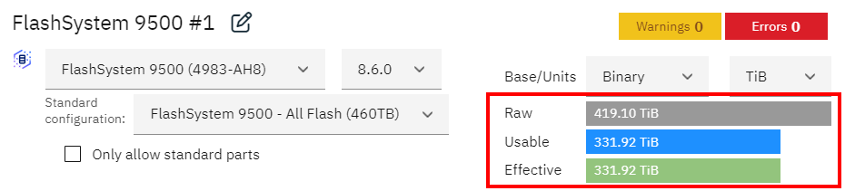
Figure 330 Capacity calculation as seen in a sample project for a System 9500
▪Raw capacity = Number of drives/modules · Drive/module capacity
– Gross capacity as marketed.
– Formerly called physical capacity.
▪Usable capacity = Raw minus overhead (RAID, metadata, reserved)
– Amount of non-reduceable (incompressible, …) data that can be stored. (Storage Modeller adds up the number of
extents available for all the drive sets that the user adds.)
– Worst case if data reduction does not give the expected savings.
▪Effective capacity = Data reduction applied to usable capacity
– Capacity that can be provided to the hosts after data reduction.
– Assumes that all savings can be achieved as expected.
An IBM task force defined new capacity definitions. With IBM Storage Virtualize version 8.3.1, the IBM Storage Virtualize and System products changed to the newly-defined capacity
terminology. For details on the new capacity terminology, see
“General Glossary for IBM Storage Modeller”.
Comparisons and examples of calculation differences
This section provides some comparisons and examples of the calculation difference between Storage Modeller and Capacity Magic. Storage Modeller precisely calculates raw and effective
capacity. These calculations are aligned with the way that IBM accounts for FCM arrays, data reduction pools, garbage collection, and other issues.
Comparison with Standard NVMe drives
In
Figure 331 on page 383
the calculation for the effective capacity using regular pool shows Capacity Magic has 218.3 TB and Storage Modeller has 74.25 TB. The difference arises here because Real-time Compression
(RtP) is not supported for the 9100, 9200, 7200 storage systems in Capacity Magic.
The calculation for effective capacity using Data Reduction Pool (DRP) shows Capacity Magic has 218.3 TB and Storage Modeller has 194.1 TB. The difference here is Storage Modeller includes
overhead for DRP, and Capacity Magic does not.

Figure 331 Effective capacity using regular pools
Comparison with IBM FlashCore Module(FCM) NVMe drives
In
Figure 332
the calculation for the effective capacity using a regular pool shows Capacity Magic has 428 TB and Storage Modeller has 424 TB. The difference here is that Capacity Magic is not aware of
the maximum IBM FlashCore Module(FCM) address space.
The calculation for effective capacity using DRP shows Capacity Magic has 926 TB and Storage Modeller has 839 TB. Again, Capacity Magic does not include the overhead for the DRP in its
calculations.

Figure 332 Effective capacity using DRP
IBM FlashCore Module(FCM) and compression
IBM FlashCore Modules(FCM) have an internal compression engine, so more data than the usable capacity can be written on a single drive. The compression is internally done in the FCM and
has a significant impact to the array algorithm.
The XLarge FCMs have a usable capacity of 38.4 TB and the maximum effective capacity is 88 TB per drive. The effective capacity is higher than useable capacity (because of the data
reduction technologies). Thus, less data can be stored before compression (38.4 TB) and more data can be stored after compression (88 TB). See
Figure 333.

Figure 333 FCM capacity
Figure 334 on page 384
includes FCM1, FCM2, and FCMn. The darker green areas are the physical usable capacity (38TB). The lighter green areas are the effective capacity (88TB).

Figure 334 FCM drives, usable and effective capacity
A 9100 array is configured in Storage Modeller with the following parameters:
▪DRAID 6
▪24 drives
▪Rebuild area: 1
▪Target grouping: 10+P+Q
▪Drive type: 38.4TB 2.5 NVMe FCM2
▪Data Reduction Pool
This configuration includes 38.4 TB usable capacity and 88 TB effective capacity per drive. As it creates the array across the whole environment, Storage Modeller uses the maximum
effective capacity of 88 TB for each drive, and the array addresses the 1.494 PB of usable capacity.
Storage Modeller then assigns the array capacity to a pool. In this example, the pool is a DRP with thin provisioning, compression, and deduplication set to zero. (Division of the maximum
effective capacity in extents minus DRP overhead.) In a DRP, Storage Modeller uses a default extent size of 4 GB allocating 592.20 TiB of usable capacity to the pool, out of the 651.02 TiB
of usable capacity at the array level. See
Figure 335.
|
Note: For drives with internal data reduction by hardware (such as IBM FlashCore Modules), Storage Modeller shows two capacity numbers for the arrays:
▪The first number (without brackets) is the array's usable capacity, that is the amount of data that can be stored even if the drive cannot achieve any data reduction.
▪The second number (in brackets) is the maximum effective capacity, that is the amount of data that can be stored if the data compressibility achieves or exceeds the drive's
designed data reduction.
|

Figure 335 Storage Modeller defined pool
You can create fully-allocated DRP volumes without any compression, allocating 592 TB of effective capacity. See
Figure 336 on page 385.

Figure 336 DRP and large FCM drives
IBM FlashCore Module(FCM) address space
This section shows how to increase the available space, using the same configuration (FCM, array and DRP) but using the space in a combined way for fully allocated volumes, and for data
reduced volumes. For example, DRP with thin provisioning or compression or deduplication set.

Figure 337 FCM address space
There is an address table with a maximum of 131.072 extents per DRP and IO group as address space, as shown in
Figure 337. The address
table contains the links from the read customer data to the extents where the customer’s data resides in a compressed or deduplicated way. This address space is limited to 131.072 extents
per DRP and IO group.
Next, a 9100 is configured with 10 drives, 1 array, drive type of 38.4TB 2.5 NVMe FCM2, DRAID6 and a grouping of 7+P+Q. At the array level, there is 236.54 TiB of usable capacity.
After the DRP reduction, there is 215.21 TiB of usable capacity. The compression ratio is 67, so there is 652.14 TiB of effective capacity defined to the pool (Figure 338). These calculations are correct and working as designed.

Figure 338 SCM, effective capacity and address space
You can run into situations where you have so many FCMs that the 131.072 extents are not enough to address the whole space. This would be the case if you had 24 drives, 1 array with a
drive type of 38.4TB 2.5 NVMe FCM2 and extent size of 4 GB. You would receive the warning shown in
Figure 339.

Figure 339 Extent limit for DRP exceeded
To resolve the address-space limitation, for the large volumes increase the extent size to 8GB, shown in
Figure 340.

Figure 340 Increase the DRP extent size to 8 GB
Data Reduction Pools and fully allocated volumes
In this example, we have a DRP with large drives and only fully-allocated volumes. With a DRP you can simulate fully allocated volumes by setting thin provisioning, compression and
deduplication to zero. We configured a 9100 array with 24 - 38.4 TB (88TB) NVMe FCM2 drive type, allocating 651.00 TiB of usable capacity, see
Figure 341 on page 387.

Figure 341 System 9500 capacity example: DRP with fully allocated volumes
If you change compression from 0 to 1%, you are changing from fully allocated Limits and Restriction to the Data Reduction Feature Limits and Restriction. (Refer to
“Defining capacity”
for details on .) As soon as you change any of the three attributes — thin provisioning, compression, deduplication — to a value higher than zero, you are affecting the usable capacity for
data reduced volumes. You will have limits that differ from those in fully allocated volumes, as in this example:

Figure 342 System 9500 capacity example, after adding a non-zero compression setting
Summary:
▪All volumes in a pool use the same capabilities (thin, compression, deduplication)
– Calculation for a mix of Fully Allocated and Data Reduced Volumes in a single pool is not possible
▪DRPs with large FCMs or SSDs are limited by address space for Volumes using data reduction features
– Volumes with data reduction features potentially cannot address the full capacity
– Increasing the Extent size to 8 GB is recommended
– Take into account the Storage Modeller warnings; see
Figure 339 on page 386
▪Consider Capacity “flip” by enabling data reduction features