Adding a workload
This section describes how to add a workload. The section includes this additional information:
Be sure to also review the orientation information in
“Performance tab (assess project performance)”.
1. Open the project. The Systems list is displayed.
Figure 103
shows a typical Systems list.
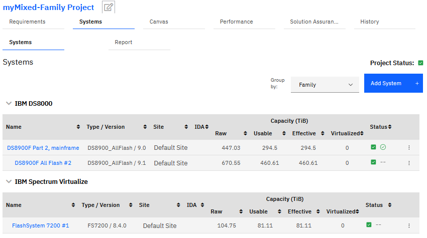
Figure 103 Typical Systems List, for a multi-family project (IBM Storage Virtualize and DS8000 families)
2. Click the Performance tab. The Workloads sub-tab is displayed by default.

Figure 104 Performance Workload page
3. Click Add Workload. The Workloads form is displayed.
All required fields are in red and must be completed before you can Save or Save and Solve the workload.
All required fields are in red and must be completed before you can Save or Save and Solve the workload.

Figure 105 Fields in the Workload form
|
Tip: While defining the workload, you might see error messages when incorrect values are entered, as shown in
Figure 106. You must correct the errors to complete a workload form. The
messages tell you what system, adapters, and capacity configurations are required to make your workload valid.
|
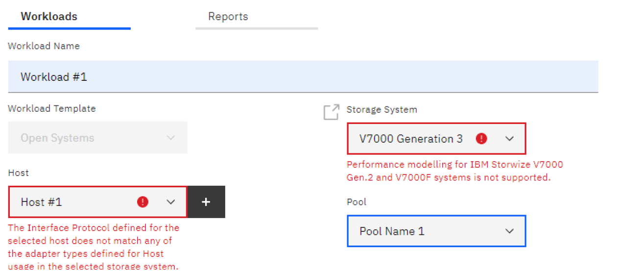
Figure 106 Error messages
|
4. Enter a descriptive Workload name.
5. From the Workload Template drop-down, select the correct template (server) to use. In late 2020,
Open Systems, IBM Z, IBM i, and
z/TPF templates were available. Future server template options are planned for Linux, OS/2, openSUSE, and Red Hat.
6. Expand the host drop-down, and select an existing host. Or select the plus-sign (+) icon to add a new host. To
learn about adding hosts, see
“Hosts tab (configure the hosts in a project)”.
7. Assign the workload to a Storage System by making a selection in the drop-down menu.
8. Assign the workload to Pool by making a selection in the drop-down menu. To the right of the selected pool, the
Effective Capacity available is displayed.
|
Note: You can define only one workload per pool. If the pool is already associated with another workload, you get an error message.
|
9. Assign the workload to a Data Space by making a selection in the drop-down menu.
|
Note: A workload can have only one Data Space assignment.
|
10. Assign the workload to a Data Space.
For background, see “Example: Adding a Data Space to pools”.
For background, see “Example: Adding a Data Space to pools”.
11. Workload Source.
– Manually entered
12. Effective Pool Capacity Used (TiB)
Enter the capacity of the workload to model.
Enter the capacity of the workload to model.
|
Note: The value that you enter in this field should always account for negative effects of garbage collection activity in NAND-* and DRP. Storage Modeller
tries to alert you to this issue during your configuration activities. In many cases, the IBM best practice is to keep 15% of the physical capacity free to allow for garbage
collection activity.
|
* “NAND-” refers to the circuitry of the memory device, which resembles a NOT-AND logic gate. NAND- is typically used in storage drives.
13. Volume Allocation.
– Fully Allocated
– Data Reduced
14. Type of Replication.
– None
– Metro-Mirror
– Global-Mirror
– z/OS Global Mirror (XRC)
– PBR Asynch
– PBR HA
For the next section, you can select the
Calculator. The Performance Statistic Calculator is displayed, as shown in
Figure 107. Enter as much information as you have available, and the calculator
automatically fills in the rest. After you fill in all highlighted fields, you can click Finish to return to the Workload form.

Figure 107 Performance statistics calculator
15. If you did not use the calculator or you want to modify values that the calculator generated, you can manually
enter the following values:
– Read I/O Percentage (%)
– Total I/O Rate (ops/s)
Tip: Enter a value from the mid-range of the I/O values that are possible in the system. That way, you generate more meaningful reports when you Solve the workload.
Tip: Enter a value from the mid-range of the I/O values that are possible in the system. That way, you generate more meaningful reports when you Solve the workload.
– Read Transfer Size (KiB/op)
(The average number of bytes read, per read I/O.)
(The average number of bytes read, per read I/O.)
– Write Transfer Size (KiB/op)
(The average number of bytes written, per write I/O.)
(The average number of bytes written, per write I/O.)
– Cache Read Hit (%)
16. (Optional) Select a value for Easy Tier Skew. Options are as follows:
None, Custom, Low, Very Low, Intermediate, High, or Very High.
Experienced users might have a
Custom value that was generated by the DiskMagic tool. If you don’t have a skew value, you might want to choose
Intermediate. In that case, a mid-range Factor value of 7.0 is automatically assigned.
Easy Tier Skew is always displayed in the Workload form. The skew setting is required, even when the pool in your original model has uniform drive types (in other words, when Easy Tier is
not active). In this way, this setting serves as a long-term reminder for when your system model changes over time. Changes might include pools moving into multi-tier drives. At that
point, you must adjust the Easy Tier Skew setting to ensure the accuracy of the model.
Figure 108
shows a set of typical statistical values for a Workload form.
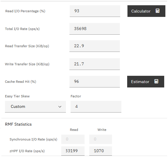
Figure 108 Typical statistical values for a Workload form
|
Note: The values in
Figure 108
include “RMF Statistics” because the example system includes an IBM z/OS mainframe. Workloads for these devices and also for the IBM Storage Virtualize devices can do data
ingestion, which is described here:
“Ingesting data into a workload”.
|
17. For the Advanced Options in the Workloads form, the model will automatically calculate based on the given
options, even when there are no values in the Advanced Options section itself. To enter values manually, expand the Advanced Option to enter Sequential (%); Random Efficiency (%);
Sequential Efficiency (%). Also see,
“About Advanced Options in the Workload form”.
18. When the form is complete, click Save to save your settings. Or click Save and Solve to populate the Reports tab with performance prediction
reports and other assessments of your workload.