Capacity / Physical Layout tab
The typical workflow is as follows:
1. In the Capacity / Physical Layout tab / Add Drive Sets Section:
Add drive sets into pool pairs on one or more frames in your system. For details, see “Add Drive Sets Section”.
Add drive sets into pool pairs on one or more frames in your system. For details, see “Add Drive Sets Section”.
2. In the Capacity / Physical Layout tab / Drive Sets Per Frame:
View the drive sets that you added and change their frame location, as needed. For details, see “Drive Sets Per Frame view”.
View the drive sets that you added and change their frame location, as needed. For details, see “Drive Sets Per Frame view”.
3. In the Capacity / Logical Layout tab:
Continue the work you started in the Physical Layout tab. View, add, and edit the pool pairing that you set up. For details, see “Editing, moving, or adding a pool pair”.
Continue the work you started in the Physical Layout tab. View, add, and edit the pool pairing that you set up. For details, see “Editing, moving, or adding a pool pair”.
For details on the physical hardware and layout display that you see in the Physical Layout tab, see
“Graphical view of frames in the Physical Layout tab”.
Guidelines for pool pairs
The following points can guide your use of pool pairs in Storage Modeller:
▪By default, you set up pairs of pools for the drive sets that you add. You can use Storage Modeller’s
Move feature to modify your initial drive-sets to pool-pairs scheme. Pool pairing follows this basic redundant formula:
– The drives in a drive set that you add to a system are always added in pairs (an even number of drives).
– Each member of a pair of drives is assigned to one of the two pools in a pool pair.
▪Pool pairing is a good architecture, but fewer pool pairs is more efficient.
Storage Modeller does not limit the number of pool pairs that you can create. That way, you are free to segregate workloads. However, keep the number of pool pairs at a minimum to maintain
efficiency.
▪The following guidelines apply when your pool pair contains multiple types of drives:
A pool pair can include multiple types of drive sets. For example, 1.6 TB High Performance drives and 1.92 TB High Capacity drives can be present in a single pool pair.
A pool pair can include multiple types of drive sets. For example, 1.6 TB High Performance drives and 1.92 TB High Capacity drives can be present in a single pool pair.
Add Drive Sets Section
The
Add Drive Sets Section
contains the
Add Drive Set button shown in
Figure 204. So, this area of the graphical user interface is the
natural place to start configuration of Capacity for the simple DS8950F Example system that is described in this document.
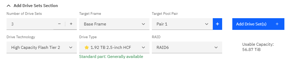
Figure 204 Capacity tab - Add Drive Set
|
Introductory points:
▪Redundancy: A key concept for Capacity is redundancy, so your addition of one drive set generates two arrays in an all- system. (There are a
few exceptions to this redundancy for systems other than all- systems.)
▪Pool Pairs: Whenever you add drive sets in the Physical Layout tab, you must assign the drive sets to a pool pair. Later, you can modify
these assignments and other pool settings, in the Logical Layout tab. Also, at any time you can add a pool pair in the Logical Layout tab and
Move drive sets into the new pool pair.
|
We do the following steps to add drive sets to the
DS8950F Example system:
1. Check the horizontal color bands in the upper right of the
Physical Layout tab. They show 0 TiB for Raw, Usable, and Effective capacity, as we would expect in a
newly created system. See Figure 205 on page 249.

Figure 205 Capacity tab - Physical layout
2. Click the caret icon (^) of the
Add Drive Sets Section, where you add and configure disk capacity as follows:
a. Set the number and type of drives for the system.
For our DS8950F Example system, we keep the default settings except for these selections, as shown in Figure 207 on page 250:
For our DS8950F Example system, we keep the default settings except for these selections, as shown in Figure 207 on page 250:
• Number of Drive Sets:
12
• Drive Type: 3.2TB 2.5-inch HPF
Figure 206 Capacity tab: adding drive sets (Callout numbers are referenced in
Table 17 on page 251.)
b. Click the blue plus (+) icon in the Target Pool Pair field (callout item
3) to create a Pool Pair to which to add the drive set. The Add Pool Pair dialog box is displayed.
For our
DS8950F Example system, the default pool pair settings are satisfactory:
• Our example system is mainframe only, so CKD storage type is
correct.
• In general, the lower option for Extent Size is recommended;
21 cylinders in this case.
• Thin Provisioning Ratio and number of volumes settings are
OK for now and can be adjusted at any time, as needed.
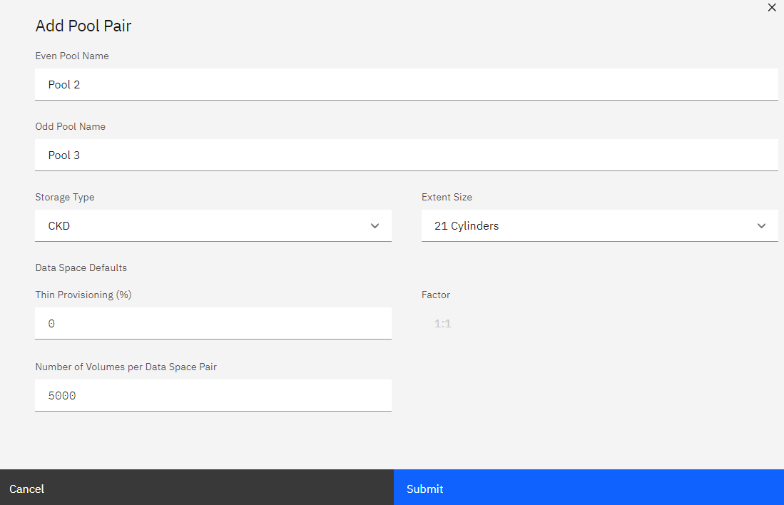
Figure 207 Capacity tab: assigning new drive sets to a pool pair
c. Click Submit. Pool pairing of the drive sets is completed.
3. Now that the target pool pair is established, the Add Drive Set +
button is active (blue color), so we click that button.
See also, “What happens when you click the Add Drive Set + button?”.
See also, “What happens when you click the Add Drive Set + button?”.
At this point, our
DS8950F Example system
already has enough detail to do performance assessments, as described in
“Basic example: Assessing performance for a DS8000 device”.
|
Tip: After you add a drive set, you might notice a configuration error or need to update settings for the drive set. You can take corrective action in the
“Drive Sets Per Frame view”
of the Physical Layout tab.
▪You can delete all drive sets through the action (vertical ellipsis) drop-down menu of the top row in this view. OR
▪Access the row for a specific drive set and choose the option you want for this drive set in the action menu:
– Edit some settings. OR
– Move the drive set to another frame. OR
– Delete the drive set, and add a new, revised one in the Physical
Layout tab. OR
|
What happens when you click the Add Drive Set + button?
When you click the
Add Drive Set + button the following events are triggered:
▪A pop-up message is displayed noting that the drive set was successfully added.
▪The color bands above and to the right of the Physical Layout tab show the actual drive space that you added, including Raw, Usable, and Effective
capacity.
▪The graphical representation of frames in the Physical Layout is updated.
For our
DS8950F Example system, all twelve 3.2 TB HPF drives are assigned to a single pool pair, Pair 1.

Figure 208 Drive sets populating a Base Frame
|
Two red boxes in the lower right of this figure highlight the following universal features of a frame view:
▪RAID6: Colored cylinder icons are drives that comprise the RAID6 (5+P+Q+S) components.
Storage Modeller displays the components of typical RAID 6: 5 green D (drive) icons, a P icon (Parity Strip1), a Q icon (Parity Strip 2), and an S icon (spare drive).
▪The red box on the left shows half of a drive set (one of two arrays in the drive set). This half is a member of Pool 0. The other half,
which is not boxed, is a member of Pool 1.
▪CKD: The red box on the right reflects the choice that you made in the Storage Type field when you
assigned the drive set to a pool pair. For our simple mainframe example, we need CKD.
For complete descriptions of features and concepts, see “Graphical view of frames in the Physical Layout tab”.
|
While you are adding drive sets, your options automatically update as you choose settings for a drive set to add.
Table 17
shows options that might be available, depending on the options you choose.
Table 17 Capacity tab / Add Drive Set Section options (Refer to callout numbers in
Figure 206 on page 249.)
|
Location
|
Callout number and field name1
|
Options
|
Comments
|
|---|---|---|---|
|
Add Drive Set Section
|
1. Number of Drive Sets
|
An integer value.
|
▪Storage Modeller pops up a message if you attempt to enter a value that exceeds the maximum number of drive sets per frame for your device.
▪A single Drive set provides two arrays and is configured for the pool pair. One array is dedicated to the even pool and one array is dedicated to the odd pool in the pool
pair.
|
|
2. Frame
|
▪Base Frame
▪Extension Frame, if applicable
|
Multiple frames are established based on your settings in the System tab.
|
|
|
Add Pool Pair dialog box (see
Figure 207).
To access, click the plus-sign (+) icon in the Target Pool Pair
field in the
Add Drive Set Section.
|
3. Storage Type
|
Select a radio button:
▪CKD (Count Key Data) - to connect to a IBM Z host.
▪Fixed Block Open - to connect to Linux, Windows, AIX, and other hosts.
▪Fixed Block IBM i - to connect to an IBM i host.
|
The DS8000 device can connect to more than one host and more than one type of storage. If you want more than one Storage Type, you must finish this configuration as one specific
type. Then add an additional drive set.
|
|
Additional settings:3
▪Thin Provisioning Ratio
▪Number of Volumes Per Pool
|
▪For CKD:
Select 21 or 1113 Cylinders
(Cylinders are a standard of measure for bytes. 21 Cylinders is close to 16 MiB and 1113 Cylinders is close to 1 GiB.)
▪For Fixed Block Open:
Select 16 MiB or 1 GiB
▪For Fixed Block IBM i:
Select 16 MiB or 1 GiB |
The drop-down menu options change based on your Storage Type
setting.
Extent Size relates to formatting the drives. Unformatted drives provide raw capacity. When drives are formatted, some capacity is used for
metadata and varies depending on extent size. The remaining capacity is called usable capacity (“usable” for writing information and data).
You create pool pairs for the drive sets that you add. Any given pool pair must use the same extent sizes, as they cannot be mixed within a pool pair. You can edit any pool pair
later, as described in “Capacity / Logical Layout tab”.
|
|
|
Add Drive Set Section
|
4. Drive Technology
|
▪High Performance Tier 0
▪High Capacity Tier 1
▪High Capacity Tier 2
▪Enterprise (available for hybrid models)
▪Nearline (available for hybrid models)
|
Selecting the Drive Technology is a balance between performance and capacity. It is most common to start with the High Performance Tier for the first Drive Technology on a
Storage Type (such as CKD). Then, as you continue adding additional drive sets (for that same CKD Storage Type), balance with a Capacity Tier. If you add a new Storage Type (such
as Fixed Block Open), the process would start again with a High Performance Tier.
|
|
5. Drive Type
|
The Drive Technology that you choose dynamically updates your options for Drive Types and RAID. The balance that you achieve between performance and capacity is affected by your
choice of Drive Technology and also by the Drive Type. For example, selecting 3.2 TB instead of 400 GB makes a large difference in available capacity.
|
||
|
6. RAID
|
5, 6, or 10, depending on the requirements of specific devices.
|
—
|
2 For CKD drive sets, an extent size of 21 cylinders is recommended. For the other two storage types, 16 MiB is recommended. These lower settings give you more usable capacity and
improved performance with some types of workloads.
3 The default settings Thin Provisioning Ratio
and
Number of Volumes Per Pool
are valid for our example. You can edit these settings later, as needed. See
“Editing, moving, or adding a pool pair”.
Table 18 Drive Technology, Drive Types and RAID (Storage Modeller automatically filters options)
|
Drive Technology option
|
Available Drive Types
|
RAID1
options
|
|---|---|---|
|
High Performance Tier 0
|
400 GB 2.5-inch HPF
|
RAID 5, 6, 10
|
|
|
800 GB 2.5-inch HPD
|
RAID 5, 6, 10
|
|
|
1.6 TB 2.5-inch HPF
|
RAID 6, 10
|
|
|
3.2 TB 2.5-inch HPF
|
RAID 6, 10
|
|
|
400 GB 2.5-inch SSD
|
|
|
|
800 GB 2.5-inch SSD
|
|
|
|
1.6 TB 2.5-inch SSD
|
|
|
High Capacity Tier 1
|
3.84 TB 2.5-inch HCF
|
RAID 6, 10
|
|
High Capacity Tier 2
|
1.92 TB 2.5-inch HCF2
|
Raid 6, 10
|
|
|
7.68 TB 2.5-inch HCF
|
RAID 6
|
|
|
15.36 TB 2.5-inch HCF
|
RAID 6
|
|
Enterprise3
|
300 GB 2.5-inch 15K
|
RAID 5, 6, 10
|
|
|
600 GB 2.5-inch 15K
|
RAID 5, 6, 10
|
|
|
600 GB 2.5-inch 10K
|
RAID 5, 6, 10
|
|
|
1.2 TB 2.5-inch 10K
|
RAID 6, 10
|
|
|
1.8 TB 2.5-inch 10K
|
RAID 6, 10
|
|
Nearlinec
|
4 TB 3.5-inch 7.2K
|
RAID 6, 10
|
|
|
6 TB 3.5-inch 7.2k
|
RAID 6, 10
|
1 RAID 5 and 10 are supported but may require an RPQ. RAID 6 is recommended.
2 Only available with models DS8884F, DS8882F and DS8910F.
3 Only available with models DS8884 and DS8886.
Drive Sets Per Frame view
Capacity information is available in the
Drive Sets Per Frame view of the Physical Layout tab. The Raw, Usable, and Effective Capacity is displayed as
a total for the Frame and for the specific drive set (see the red boxes in
Figure 209 on page 254). After entering the modeling
information needed in Add Drive Set Section, data is automatically populated into the
Drive Sets Per Frame section and more functions are then available there, such as Edit,
Move, and Delete.

Figure 209 Drive Sets Per Frame view.
Click the caret icon (^) beside Drive Sets Per Frame to access the summary report and to use the available
action icons, which are both visible in Figure 209:
▪Use the action icon (vertical ellipsis) to the right of a Base Frame row or an Expansion Frame row to delete all drive sets within that frame.
▪Use the action icon for a specific drive set line to Edit, Move (to another frame) or
Delete that drive set. The Edit Drive Set dialog box dynamically displays the following options, which are
fully described in Table 17 on page 251:
– Number of Drive Sets
– Frame
– Target Pool Pair (Storage Type and Extent Size)
– Drive Technology
– Drive Type
– RAID
|
Note: You can move a drive set from frame to frame by selecting Move from the action icon on the drive set row. The
Move option is grayed out if your system has only one frame.
|
Graphical view of frames in the Physical Layout tab
Located at the bottom of the Capacity view is the physical hardware and layout section. It is a graphical representation of the physical aspects of the Base Frame and any Extended Frames.
Inside the Frames are the Enclosures that hold the drive sets and spares. The logical aspects of the system (such as pool pairs) are not directly represented, as they are not physical
hardware.
The purpose of this section is to allow customization of the physical layout of the Base Frame and any Extended Frames. Customization is usually done for performance reasons. Though
capacity can be affected by changing the layout and increasing or decreasing spares, the significant factors in customization are managing performance and cost. For example, having two
drive sets in an enclosure pair means that enclosure pair is more highly utilized than an enclosure pair with a single drive set. Enclosure pairs that are utilized less have a higher
margin of performance. However, each enclosure pair increases the cost of the Base Unit.
Utilization can be minimized if the data that is served by the multiple drive sets is not hot. So even though one should proceed with caution when not using the default Base Unit setup,
customization is available for the purpose of balancing cost, utilization and performance. Customization may require an RPQ.
Figure 210
shows an overview of the Graphical display for the Physical Layout.

Figure 210 Physical Layout Overview
The Graphical view of the Physical Layout section provides the following options:
– Save as Image: This capture function creates and downloads a
.png image of the Base Frame and any Extension Frames.
– Allow HPFE Intermix
checkbox: Allows drive sets of the same Drive Technology to be located in the same enclosure pair. High Performance (HPF) cannot be located in the same enclosure pair with High Capacity
(HCF). A variety of HPF options can colocate, as well as HCF with HCF options to reduce the number of needed enclosure pairs.
– Number of HPFE Pairs: You can vary the number of HPFE pairs depending on
the model of DS8000 that you have selected, the number of cores, and the system memory. These factors combine to determine the maximum capacity and number of enclosure pairs. The number of
pairs is also affected by the number of drive sets assigned. For example, if you have only four drive sets, you cannot select eight enclosures even if that option is displayed in the
drop-down menu.
– (Graphical display of the physical layout): The graphical display of the
Base Frame and any Expansion Frames updates dynamically to reflect your configurations. The default Base Frame is displayed with the Default option displayed
in the Number of HPFE Pairs drop-down menu. To customize the Physical Layout, change either or both of the following attributes:
• Select a number in the
Number of HPFE Pairs
drop-down menu.
• Select the checkbox for Allow Intermix
Your changes automatically generate updates to the graphical displays.
Figure 210 on page 255
shows a default layout for the Base Frame. The same configuration of drive sets is used in
Figure 211 on page 257, however the Base Frame has been
customized. The number of HPFE Pairs is changed to 4. The Base Frame is dynamically changed to its new layout. Also notice that a warning has appeared
notifying that an RPQ may be required.
Figure 211 on page 257
shows a customization change to the Base Frame for the number HPFE Pairs.

Figure 211 Customized layout for the Base Frame and its number of HPFE Pairs.
Figure 212 on page 258
shows the customization of the physical layout by checking
Allow Intermix to use fewer enclosures. Clicking Allow Intermix dynamically changes the Frame. A warning that an RPQ may be required is
displayed and will disappear if you return to the default setup.

Figure 212 Customization of the Physical Layout using Allow Intermix