News
Abstract
You can analyze a day's worth of performance data in graphical views with Collection Services and Performance Data Investigator (PDI). You can monitor live performance data graphically with System Monitoring and PDI. Starting in IBM i 7.3 release there is historical data support with Collection Services as well as graphical display of that data with Graph History in the Performance task of IBM Navigator for i (PDI).
Historical data can help you identify trends and investigate performance issues from the past or to compare today's performance with a time period in the past that you select.
Content
Historical data
Collection Services keeps up to 24 hours of data in each collection. By default, the collections are preserved on a system for 10 days. Users have a need to look at performance data and compare from week to week, month to month, or even year to year. So it was necessary to provide a way to keep performance data for longer periods, without taking up too much storage. Another requirement is to allow an easy way to view data across multiple days.
This is handled by the Collector with the new Historical Data collection. The new performance collection type *HSTFILE contains historical data in a file-based performance collection.
The Historical Data collection is data collected by Collection Services that is reduced and summarized to keep the data over a long time and conserve space. The data is intended to be just a subset of the original Collection Services data.
The Historical Data collection is populated with data from management collection objects in the configured collection library (for example, QPFRDATA) when the Collection Services collector is cycled or ended.
To enable the concept of aging or decaying data, there are two levels of historical data – detail and summary. As you can see from the following table, as the maximum collection duration increases, the number of metrics available decreases.
Table 1: Collection data duration and variety
The summary historical data is the system-level and summarized metrics. This data is useful in identifying trends or detecting changes in a system over a long period.
The detail historical data is the collected data saved for top contributors of each interval, as well as other relevant supplementary data. The detail data is the supporting data for the summarized metrics. The detail data can be used to delve deeper into a problem identified by summary historical data. Only the top contributors for each metric are stored as historical detail data.
Create historical data on IBM i 7.3 or later
To turn on the creation of historical data on an IBM i 7.3 or 7.4 partition, use the Collection Services configuration panel. Under the Performance task on IBM Navigator for i, click Configure Collection Services.
Figure: Configure Collection Services
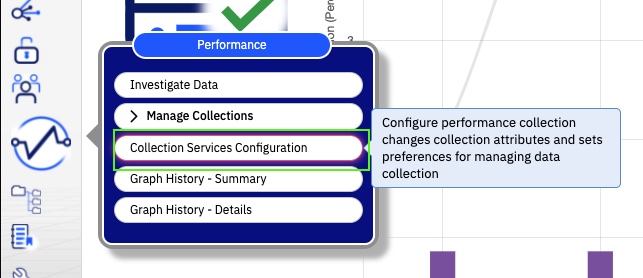
Figure: Option to create historical data
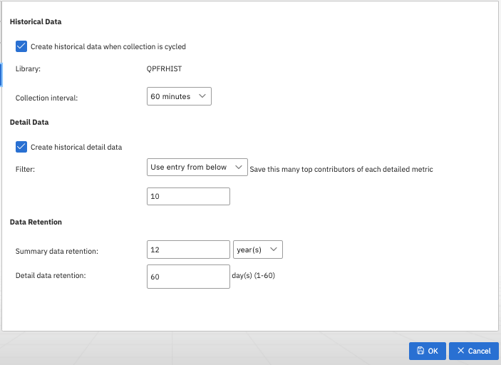
- On the Historical Data tab, select Create historical data when collection is cycled.
- For the Collection Interval, you can specify the historical data interval (default is 60 minutes). The summary and detail historical data is saved in the Historical Data collection at this requested interval.
- For Data Retention, you can specify the length of time that historical data is kept. Up to 60 days of detail historical data and 50 years of summary historical data is kept by Collection Services; with defaults being 7 days and 1 year.
Table 2. Historical Data retention
You can use the additional options to configure historical detail data:
- Create historical detail data
You may create only summary historical data or both summary and detail historical data. The default is to create historical detail data when summary historical data creation has been selected.
- Detail data filter
The detail data filter determines what number of top contributors for each metric is stored in the detail data files. The top contributor means the job or task, disk, memory pool, or communication line that had the most significant values (CPU %, response time, utilization, and so on) during that interval. Only data for these top contributing elements is saved as historical detail data for that interval. The default is that 20 top contributors for each metric at each interval is stored.
Set the options, then click OK.
With these configuration options in place, you can create historical data for any *MGTCOL objects in your configured library by selecting to "Cycle" the Collector. For this, go to the General tab
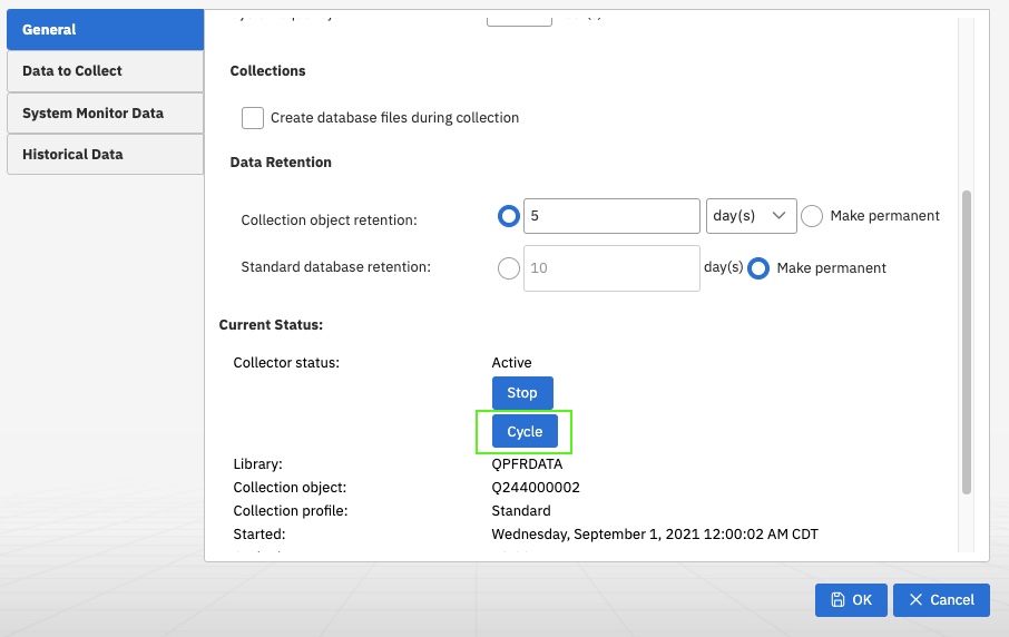
Cycling will cause the data available in the default library to be put into an initial historical data file used to view the Graph History charts.
Creating historical data from existing collections
When you turn on historical data creation, the next cycle of Collection Services will cause all available data in *MGTCOL objects within the configured library to be used to create the Historical Data collection. You can also manually generate historical data from other *MGTCOL objects by using the Create historical data action in Manage Collections.
Visualizing historical data with the Graph History function
After the historical data is created, use the Graph History function in the Performance task on IBM Navigator for i to view historical performance data. As mentioned earlier, this enables you to view data over long periods of time, from days and weeks to months and years. The Graph History function provides access to the new Historical Data collection, both summary and detail performance data.
Graph History Summary charts
Historical Summary charts leverage the historical summary data to provide single metric charts to view and analyze performance over the selected time span. The metrics provided in the summary charts focus on the system monitoring data saved into historical data. From the Summary chart, the top contributor information from the historical detail data for that metric is available by selecting an interval. From that Top Contributor chart, the property data for a top contributing element is available by selecting the element.
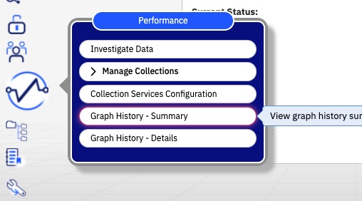
To view the historical data, use the new Graph History task section in Performance. To start, select Summary under Performance → Graph History.
Figure 9. Summary action
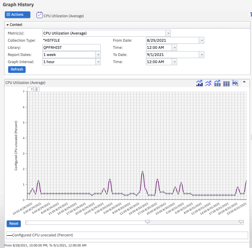
This Historical Summary chart shows the CPU utilization (average) for 1 week with 1-hour intervals:
Zoom in
When the chart is first displayed, it displays the data for the past month at one hour intervals. Many times this is too many points to clearly distinguish each interval on the chart, so the chart will display as a line without plot points. As you zoom in, the individual data points are shown.
To zoom in a specific point or time interval, you can use the slider or the mouse wheel.
To use the mouse wheel, click the data point on the graph for the interval area that you want to zoom in, then use the mouse scroll wheel to zoom in.
Figure 12. Slider
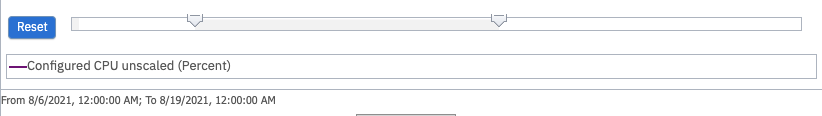
To return to the chart as it was originally presented, click Reset.
Figure 13. Tooltips
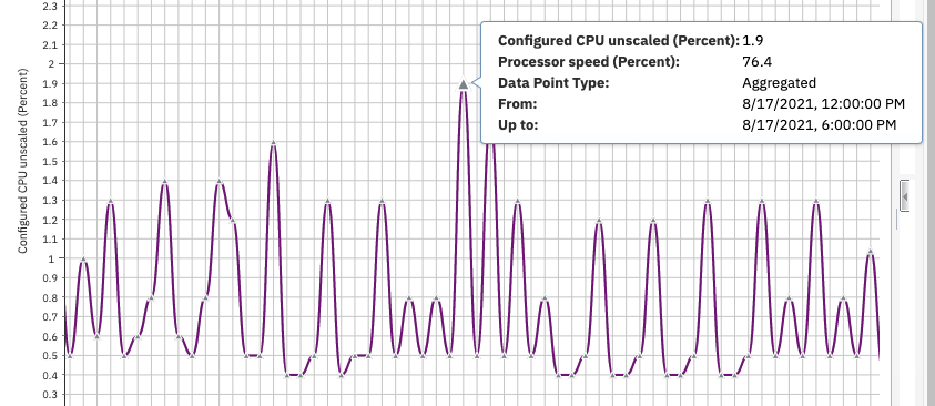
As you move the mouse pointer over the plotted points on the graph, tooltips appear with the value charted and other detailed metrics about each interval data point.
Figure 14. Icons
The five icons at the upper-right of the chart can be used to modify the presentation of the panel. The options are as follows:
-
Chart view – (default) Select the chart icon to view the data on the chart.
-
Stacked chart view - Compare the data points against other days, weeks, or months
-
Chart & Table view – Select the combined chart and table icon to split the screen between the graph and the table.
-
Table view – Select the table icon to show the data set only in table format.
-
SQL – Select the SQL icon to display the query used to obtain the data set charted on the graph.
Figure 15. Maximum graph value
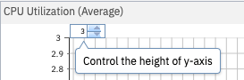
Use the maximum graph value dial to zoom in the chart by changing the graph range (maximum graph value) shown on the chart. Points that are larger than this setting will not be seen on the chart.
Context panel
When the Summary chart is first displayed, it shows data starting from today's date in the previous month up to today. Use the Context panel to select any other available metric to be displayed.
The Context panel is closed when the chart is displayed or updated to provide more room for the chart. Expand Context to open it.
Figure: Context panel
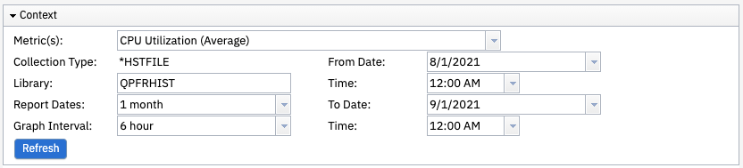
Use the Context panel to view and modify the chart specifics such as metric, report dates, graph interval, and dates.
After any changes to the Context panel, click Refresh to update the chart with the new settings.
Use the Metric drop-down list to switch to any of the other available Historical Summary charts. Other settings of the Context section such as graph interval and dates are preserved when selecting another metric to display.
The Collection Type is *HSTFILE.
The default Library is QPFRHIST. Change this field to another library if you copy or move a Historical Data collection.
The time span displayed on the graph is determined by the Report Dates field.
The Graph Interval values available are based on the Report Dates range. For a larger range of time, the graph intervals available are larger. For a smaller range of time, the graph intervals available are smaller. For example, if one month of data is requested, you are able to set the graph interval to 1 hour, 6 hours, 12 hours, or 1 day (24 hours). If a report date greater than one year is chosen, then the graph interval values available are one month or one year. Table 3 shows the Graph Interval settings available based on the selected Report Date range.
Table 3. Report dates and graph interval settings
Use the From Date and Time fields and To Date and Time fields to select a custom range (report date) to be displayed.
The Historical Summary chart initially displays data starting from one month ago and ending with the collection last ended (often at the default midnight cycle time). To modify the dates and times displayed, first modify the Report Dates field or change the From Date and Time fields and To Date and Time fields. Then, select a Graph Interval value and click Refresh.
To view historical data collected today, you must manually generate historical data for the active Collection Services *MGTCOL collection by using the Create historical data action in Manage Collections.
Understanding the Historical Summary chart
The Summary chart is created for one metric over the specific time range selected in the Context section. Each point on the graph is shown with a symbol and color, which indicates information about the data charted at that time interval.
A circle represents a data collection point that has historical summary data available, but no detail data available.
A square or triangle both represent data collection points that also have historical detail data available. You can click a square or triangle icon to see the top contributors data for that interval. The Top Contributors chart appears at the right side of the Graph History window.
The outline of the data point symbol also indicates information about the data being charted. The data point is collected, aggregated, or extended.
- A collected data point is a value taken directly from a historical database file.
Figure 18. Collected data point
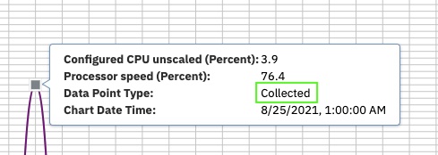
The historical data requested interval and graph requested interval match at the highlighted data point.
- An aggregated data point is a calculated value from the metric at multiple intervals in the historical database files. Aggregation is done when the collected interval is less than the requested graph interval. Calculations such as sum, average, or max are performed depending on the metric and what it represents.
For example, if data is collected at 15-minute intervals and the chart is showing 1 hour graph intervals, the data point is a calculation of metrics from 4 time intervals.
Figure 19. Aggregated data point
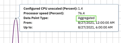
The historical data requested interval is smaller than the graph requested interval at the highlighted data point.
- An extended data point is a value for that time interval, which is not available in the historical database file. The data value is extended from the last available interval value. The extended data points are needed to provide integrity to the chart for the graph interval requested.
For example, if data is collected at 30-minute intervals and the chart is showing 5-minute graph intervals, the data points between the collected intervals are extended.
Figure 20. Extended data point
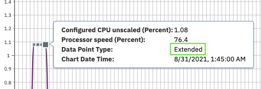
The graph request interval is smaller than the historical data creation requested interval at the highlighted data point.
Top Contributors chart
To view top contributor information for an interval, the detail data needs to be available. The detail data is indicated by a square or triangle plot point. Select the data point. The Top Contributors chart is displayed at the right side of the panel.
Figure: Top Contributors chart
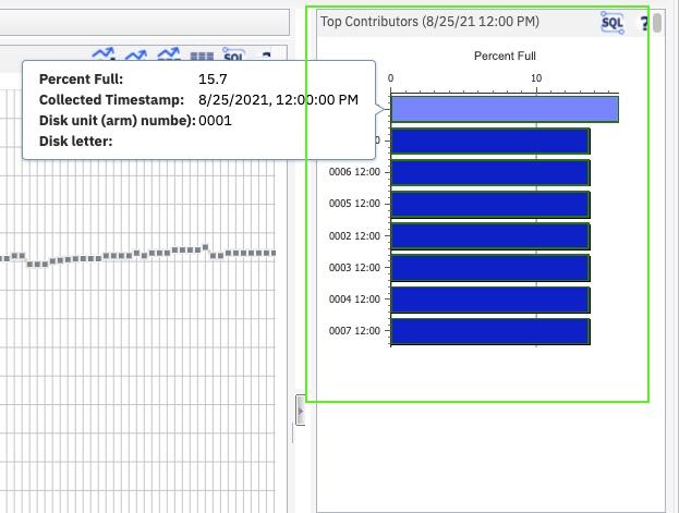
This chart shows the top contributors for the temporary storage in the selected time period. If a disk, job, or pool is a top contributor for more than one interval of an aggregated data point, it can be listed multiple times. (See aggregated data point.)
For example, the triangle data points indicate where the data was collected at 30-minute intervals but a 1-hour graph interval was requested. There can be duplicated job, pool, or disks because they happen to be top contributors for both intervals. For an aggregated data point, both values are included in the calculation for a requested interval. The time stamp on the Top Contributors chart helps to differentiate them.
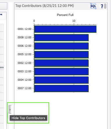
To resize this section, click the Hide Top Contributors button.
Figure 24. Hide Top Contributors
Property data
From the Top Contributors graph, you can view property data for a job or task, memory pool, disk unit, or communications line by selecting a bar from the Top Contributors graph.
The Properties panel appears under the Top Contributors chart.
Figure: Properties panel
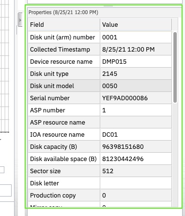
The Properties panel contains all the information available for the job or task, communications line, memory pool, or disk pool. You can scroll down the panel to see all the fields.
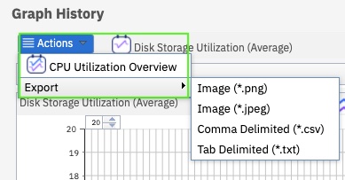
Actions menu
- Use the Actions menu to open the Historical Detail charts. l
- You can also export the Graph History charts as an image, text, or csv file
Figure 27. Actions menu
Graph History Detail charts
The Historical Detail charts provide a view of more data beyond the single metrics provided in the Summary charts. The Detail chart uses multiple summary metrics to provide more information at each interval. Some of these are similar to well-used PDI perspectives.
From the Detail chart, the top contributor information for one metric is available by selecting an interval. From that Top Contributor chart, the property data for a top contributing element is available by selecting the element.
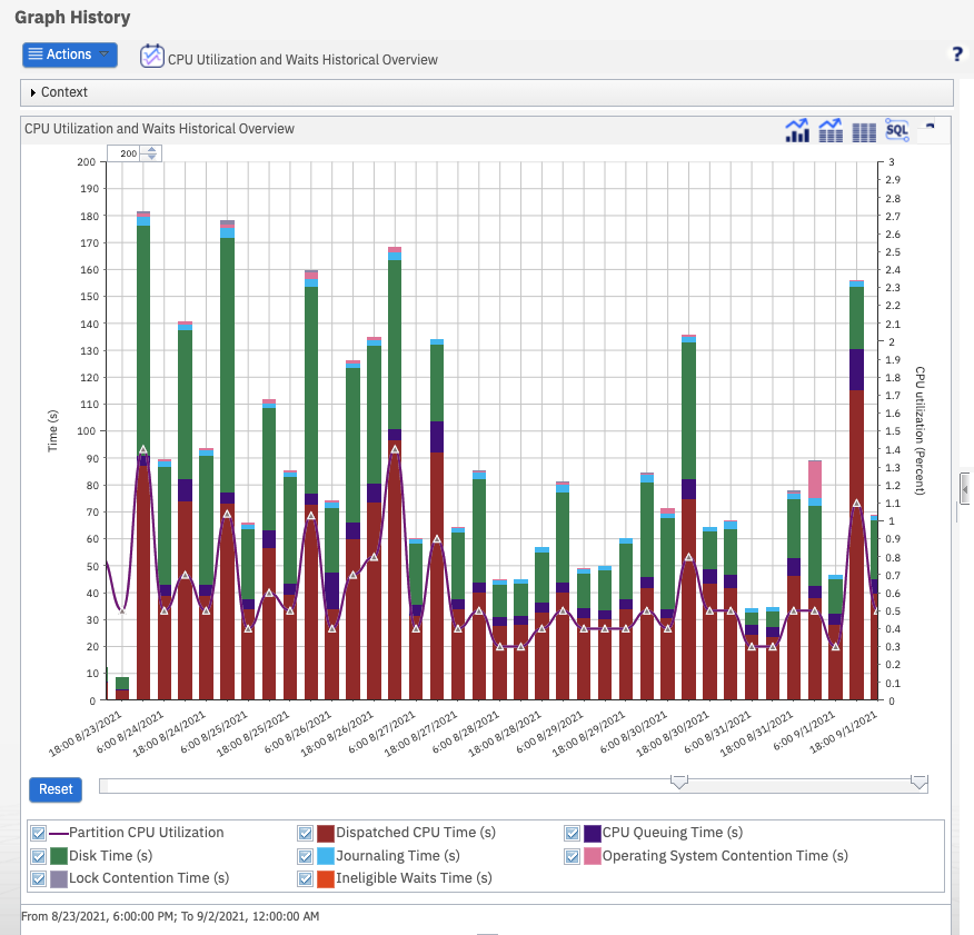
The CPU Utilization Overview Historical Detail chart provides the Partition CPU Utilization and CPU time used from the summary data. When you select a point and drill down to top contributors, the metric analyzed is CPU time charged to the job.
Requirements
Historical Data and the Graph History analysis tool is included with the base operating system in IBM i 7.3 and later releases.
PTF requirements
For best results, make sure you have the latest Group PTF level for IBM HTTP Server for i installed on your system:
User profile authority requirements
To access the historical data, a user profile needs to have *ALLOBJ authority or be included in the data authority list QPMCCDATA for access to the Collection Services data.
A user profile needs to have *JOBCTL authority or be included in the function authority list QPMCCFCN to use the performance commands in IBM Navigator for i. You can only run Configure and Cycle Collection Services and access the Performance Tools functions when your user profile has the correct authority. See Authority for more detail.
Summary
We can't predict the future. We can't guess today what your system performance is going to be tomorrow. However, with this new Graph History function, you can look back in time and better analyze your system performance over a long term. Anticipate future performance with this tool. Turn on historical data now and in the future you can examine past system performance. Use PDI Graph History views to gain hindsight tomorrow for what is happening on your system today.
Was this topic helpful?
Document Information
Modified date:
30 September 2021
UID
ibm16217189