How To
Summary
Use pGraph from Federico Vagnini (IBM Italy) is a flexible Java tool for graphing many data sources.
Steps
pGraph is a Java program designed to read multiple performance data formats and to produce graphs either interactively or in batch mode. There is no limit on input data size and user can view graphs related to the entire timeframe or can select a specific time period. Only requirement is a JRE 1.5 or newer.
For quick overview see 20250204_hmcScanner_pGraph_1.pdf
pGraph major features:
- support for multiple data formats (nmon, vmstat, topasout, iostat, lslparutil, sar)
- multiple operating systems (AIX, Linux, Solaris, HP-UX)
- no limit in performance data file size
- data file can be in GZIP format (highly recommended to save space)
- can read multiple files at a time
- automatic merge of data files belonging to same operating system
- load of files belonging to multiple operating systems to show global processor usage
- complex mixing of data is possible (e.g. 100 LPARs, with 7 nmon files each)
- zoom feature to show data related to a user defined time period
- graphs can be exported in PNG or CSV format
- applet version for easy web publishing
- simple capacity planning feature
The tool is constantly updated to match changes in tool syntax, to manage new data types and to add new features. If you have any problem or any suggestion to improve pGraph, please send me a mail (vagnini@it.ibm.com). Since new features are mostly suggested by users, propose yours!
pGraph is packaged in a single Java jar file available in the download section of this page.
This tool is not officially supported by IBM. No guarantee is given or implied, and you cannot obtain help from IBM. It a personal project of the author, Federico Vagnini (IBM Italy).
See also HMC Scanner page from the same author.
Input data
pGraph can read data from several performance tools. Just save the text output of the tool on a file with the name you prefer. In order to save disk space, it is possible to compress the text file in GZIP format with a ".gz" extension. pGraph will automatically detect the file format and load the data. There is no limit in file size or in the number of samples present in the data.
Supported data formats
pGraph can be easily adapted to read the output of many performance tools, provided they print a time stamp for each data sample. The following table shows the current tools supported:
| Command | AIX | Linux | IBM i | Solaris | HP-UX | |
|---|---|---|---|---|---|---|
| nmon (raw output, unsorted) | X | X | ||||
| vmstat -t | X | |||||
| topasout (any source, for example xmwlm, topas_cec) | X | |||||
| iostat -alRDT | X | |||||
| HMC's data collection using "lslparutil" command | X | X | X | |||
| sar -A | X | X | X |
NOTE When using sar on Solaris or HP-UX no information is provided about the number of available cores. If you want pGraph to provide an estimate of real process consumption (as if the technology could provide a capability similar to the one available on IBM PowerVM), add a single line at the beginning of the file with the syntax "cores = number_of_cores.
Single and multiple file load
The following features are available:
- Load from single file
- single data file
- single host, multiple files : files related to the same operating system that need to be merged
- multiple hosts, multiple files : each file is related to separate operating systems and you want to compare them
- you can mix the previous cases and perform additional operations on data
When a single file is selected, pGraph automatically detects its type and parses it. When the file is completely loaded, a set of graphs are made available, depending on the file content (for example, iostat does not provide CPU data).
The same performance tool can be run several times (for example, an nmon running every day for 24 hours) on the same operating system and the administrator may need to study all the outputs. pGraph is capable of automatically merge the content of files and treat them as a single input stream: just put all files in the same directory and load them with the single host, multiple files option. There is no requirement on file names since pGraph will use time stamps inside the files to correctly merge data. This feature does not apply to vmstat and iostat files that provide only time and not date: in this case concatenate the files by yourself in the right order and load the result (e.g. cat file1 file2 file3 > concatenated-file).
When an administrator collects data from several operating systems it may become very useful to compare how they are working in the same time period. pGraph can extract CPU and I/O data from each file, align in time all samples, show graphs related to each operating system and provide additional graphs that show the sum of all workloads. When nmon is used and all operating system are hosted by the same partitioned system, global processor pool and sub pool statistics are also available. To obtain this view, put all files into the same directory and load it with the multiple hosts, multiple files option.
Sometimes administrator has complex analysis to made involving many files (maybe hundreds of them) with multiple views to made. In order to provide a very flexible file load schema, administrator can use a configuration file to program how pGraph loads files. A configuration file can use a mix of files and directories, select a specific timeframe to show and even apply multipliers to CPU consumption to make simple capacity planning. The syntax is very simple:
| Command | Description | |
|---|---|---|
| # | Every line staring with "#" is considered a comment and is ignored | |
| BASE = <directory> | Base directory for relative paths in following lines. It must be and absolute path. | |
| SH_DIR = <directory> [@ weight] | Directory containing files belonging to the same operating system that must be merged. The optional weight is applied to all CPU consumption data. | |
| MH_DIR = <directory> [@ weight] | Directory containing files belonging to multiple operating system. The optional weight is applied to all CPU consumption data. | |
| <file> [@ weight] | File containing performance data. The optional weight is applied to all CPU consumption dat. | |
| ZOOM = YYYYMMDDhhmmss - YYYYMMDDhhmmss | Time period to start with in graphs. |
The following is a commented example of a configuration file:
# Base directory containing all nmon data. All following directories are BASE's children BASE = "C:\pGraph data\080220-SCON" # Directory containing multiple nmon files related to the same LPAR: concatenate them # Apply a scaling factor of 0.74 to all CPU consumption data SH_DIR = 690_1_090 @ 0.74 # Two directories, each containing only one nmon file for each LPAR. Apply two separate scaling factors to CPU usage MH_DIR = 595_1 @ 0.5 MH_DIR = 690_1 @ 0.74
Simple capacity planning
The weight parameter available using configuration files is useful when you want to perform simple capacity planning on CPU and you want to estimate how many cores you need on a micro partitioned IBM Power System.
Collect real workload data for the time period you like (it may be the length you want) on all the operating systems you want to study. The operating systems may be hosted by multiple hardware systems but they must be collected in the same time period. This is the base workload.
Decide if workloads will have or not a growth in CPU consumption and then decide the target IBM Power System that will host all workload with a micro LPAR for each operating system. This two changes must then be reflected in a weight factor to be applied to current CPU usage. pGraph will scale base workload by the provided factor and show you each workload and the combined consumption. The result will be a simulation of the sum of workloads in time that allows you to evaluate the real needed capacity, exploiting the full capabilities of IBM PowerVM.
If a workload is currently hosted by a dedicated hardware or partition, pGraph will apply the average User+System percentage data to the number of cores available to evaluate a reasonable amount of physical CPU used "as if" the workload were hosted by a micro LPAR on an IBM Power System. This data can be extracted even from sar files coming from Solaris and HP-UX.
The weight factor is the critical element in this type of analysis. There are several ways to identify it and you can apply any contingency you want:
- Migration from IBM Power to IBM Power: use rPerf values that IBM publishes and keeps updated on System Performance Reports
- Migration to IBM Power from another hardware system: perform a specific application benchmark or choose a similar benchmark to define the value.
- Contingency: this computation is never exact so you may want to add some additional capacity
Example 1: Your workload will grow by 20% and the target system has 50% more rPerf than the source with the same number of cores. Weight = 1.2 / 1.5 = 0.8, meaning that the workload will use on the target system 80% of physical cores it is using on the source system. If you want to add 10% contingency, the weight to be used with pGraph is then 0.8 * 1.1 = 0.88
Example 2: Your workload is running on a dedicated UNIX system and will be moved to an IBM Power System. You have detected that there is an average scaling system of 2.5 in core consumption when performing such migration. The pGraph weight will then be 1 / 2.5 = 0.4.
pGraph execution
pGraph only requires a Java virtual machine (JRE or JDK) version 1.5 or later, so it can be executed almost everywhere. It can be run either in interactive mode, in batch mode or in applet mode.
When dealing with performance data that include many objects (cores, disks, adapters, top processes), the default memory configuration of Java virtual machine may cause out-of-memory errors. In this case you must increase the memory available to Java. This is normally done on the command line by using the -Xmx<size> parameter (e.g. java -Xmx500m to allow up to 500 MB of memory).
You can change some pGraph default values by creating a pGraph.properties file and placing it in the same directory the pGraph.jar file is. pGraph will read the file only once when it starts and update itself according to the file content. A sample properties file is provided in the download section.
Interactive mode
If your operating system has associated the "jar" extension with a JVM you can just use the GUI and double click on the pGraph.jar file to launch the program. If you prefer command line (you still need a graphic environment), the syntax to run the tool is (case sentitive):
java -cp pGraph.jar pGraph.Viewer [input file]
If you do not provide an input file on the command line, the pGraph GUI will start with an empty workspace waiting for your input file:
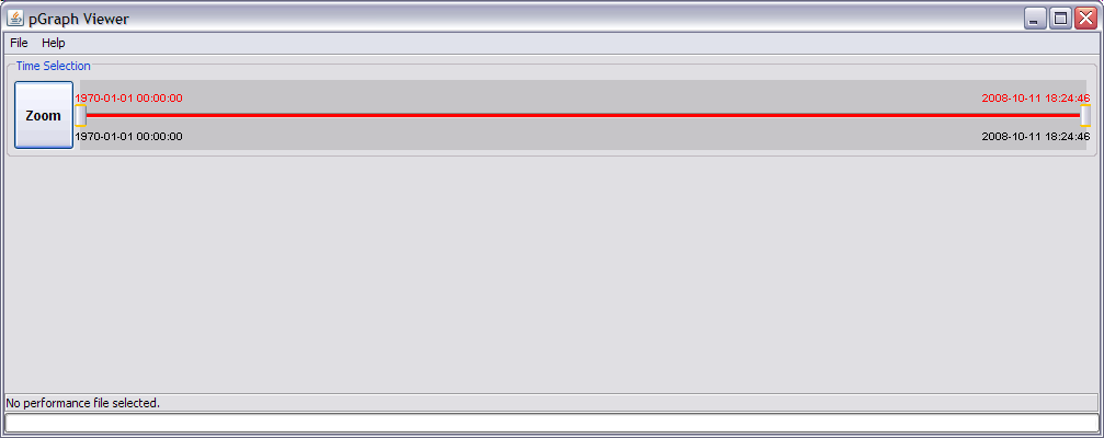
Use the Help menu to access to the tool's Console with all error messages or to the About panel that provides the version of the tool you are using.
The File menu is used to select the file or the directory to be loaded. A separate window will appear allowing you to navigate inside your local filesystem. Once you select the data source, the tool will show on the lower part of the GUI the status of file loading up to completion of data parsing. pGraph will first scan the file to detect its format and to identify the time range contained into the file(s). During this period of time you will see a bar moving back and forth. Once pGraph identifies the source type, it will start parsing the data and you will see a progress bar showing the percentage of lines read. If multiple files are read (either after the selection of a directory or a configuration file), the progress bar show the percentage of each single file read.
If you have provided an input file with the command line, it will be loaded immediately as if you selected File -> Load single file.
When parsing is complete, the GUI is updated showing the timeframe contained in the file(s) read and a set of buttons. Each button can be pressed to create a new window containing performance graphs. The number and types of buttons depend on the source file(s) type. Pressing a button may cause the creation of an empty window: in this case no data in the file was present that could be used to create the required graphs. If errors occur during graph creation, a console window will pop up providing some hints on the error cause: try to check the source file for errors or report the bug sending a mail to vagnini@it.ibm.com with the description of what you made and, possibly, a GZIP version of source file(s).
For example, when a single nmon file is loaded, the GUI looks similar to the following:

All graphs will be always related to the timeframe shown in the GUI. If you need to focus on a restricted time window, perform a Zoom operation and pGraph will re-read the data source and update all graphs.
Batch Mode
The tool can be used in batch mode to create PNG pictures of all available performance variables (the same PNG of interactive mode) with an HTML wrapping that can be used to publish them on a web site.
Due to Java limitations, a graphical adapter or a virtual frame buffer is required.
The syntax for batch mode is:
pGraph.Viewer - Version 2.0 Interactive Usage: pGraph.Viewer [file] Batch Usage: pGraph.Viewer [ -l begin end ] [ -d | -D ] <source> <output dir> -l limits time frame: begin and end in YYYYMMDDhhmmss format. -d source=directory : multiple hosts in multiple source files. -D source=directory : single host with multiple source files. <source> is by default a file. Use -d or -D to select a directory. Valid input files are: "nmon", "vmstat -t", "topasout <xmtrend file>", "topasout <topas_cec>", "iostat -alDT", "lslparutil" <output dir> is where system usage reports in PNG format are written.
By default the entire time period contained in the file(s) is examined, but user can change it using the "-l" switch.
If multiple input files are available, place them in the same source directory. If they belong to the same operating system, use the -D switch and pGraph will merge them providing all contained information. If the files belong to different operating systems and a global view of CPU usage is required, use the -d switch and pGraph will provide a CPU graph for each file, all related to the same timeframe.
In the output directory, a PNG picture is created for each available graph. For web publishing, an "index.html" frame is provided to ease browsing among pictures.
For example, a complete HTML/PNG report for file myServer.nmon can be created inside directory report with the following command:
java -cp pGraph.jar pGraph.Viewer myServer.nmon report
A virtual frame buffer can be set up in the following way:
AIX
- Install the X11.vfb fileset
- Start the X server: /usr/lpp/X11/bin/X :1 -vfb -force -x abx -x dbe -x GLX & >/dev/null 2>&1
- Export the display: export DISPLAY=1:0
Suse 10.4
- Install the package xorg-x11-Xvfb-6.9.0-50.80.1
- Start the X server: /usr/X11R6/bin/Xvfb :1 -dpi 96 -screen 0 800x600x24 & >/dev/null 2>&1
- Export the display: export DISPLAY=1:0
Applet Mode
NOTE: Modern browsers will not allow you to execute applets that are self signed like pGraph.
If you have an HTTP server that provides access to performance files, you can use pGraph's applet version to allow users to download the files and interactively analyze then as if they were on the local filesystem. The applet provides the same GUI and the same functionalities as in the interactive version, but it will have access only to the files you define in applet configuration. The pGraph.jar file is signed using a self-signed certificate: if the user accepts the certificate, the applet will be apble to run correctly and to produce PNG pictures of performance graphs on the user's local filesystem.
The pGraph.jar package contains the pGraph.ViewerApplet class that can be used in the HTTP server. It will show by default on the web page as a button with a Start label. If you want another label, it can be customized. When the button is pressed, the applet will create the GUI and start downloading from the server all the performance files associated. Since network is used, it is highly recommended to store performance files compressed in GZIP format with a ".gz" file extension.
The applet accepts three possible parameters:
- FILES a comma separated list of files on the web server that will be read by the Viewer. The path is either relative to the jar location or a full URL
- SINGLE_HOST true or false value
- LABEL label to be printed inside the applet in the web page. The default is Start
FILES parameter must be used otherwise the applet will be empty with no chance of loading any file. The Viewer will immediately load the provided files from the web.
If FILES containes a single file, tha applet will show its content. If FILES contains multiple files, they will be treated as belonging to multiple servers and only CPU data will be shown (like in multiple hosts, multiple files), except when SINGLE_HOST is set to true value. The SINGLE_HOST parameter should be used when multiple files belonging to the same operating system are provided and must be merged by the applet.
Examples of usage: single nmon compressed with GZIP, three nmon files to be merged:
<applet code="pGraph/ViewerApplet.class" archive="pGraph-1.5.3-alpha.jar" width=80 height=30 files="files/nmon.gz"> </applet> <applet code="pGraph/ViewerApplet.class" archive="pGraph-1.5.3-alpha.jar" width=80 height=30 files="mfsh/nmon1,mfsh/nmon2,mfsh/nmon3" single_host="true" label="mfsh"> </applet>
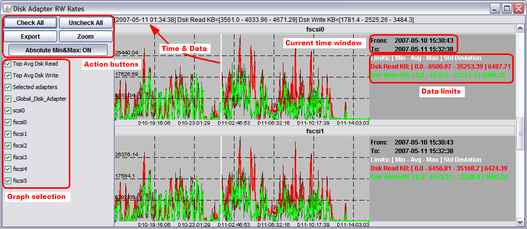
Graph window components
All graph windows have the same components, as shown by the following picture:
- Action buttons
- Graph selection
- Time and Data
- Current time window
- Data limits
- A set of performance graphs
By default all available graphs in the window are selected and shown. Each one has a title that is also present in the graph selection area. Each graph can be hidden or shown by acting on the corresponding check box in the graph selection area.
The Check All and Uncheck All buttons are shortcuts to select or deselect all graphs at once.
The Export button allows to export all the selected graph on the local filesystem as a single PNG picture (default) or as a text file in CSV format. A file selection window will appear to select filename and directory. In order to export in CSV format, change in the file selection window the file type. CSV format can be loaded by a spreadsheet but in order to simplify my language requirements (I'm Italian), fields separation character is a semicolumn and decimal separator character is a dot.
The Zoom button is used to change the current time window, as described in the following section.
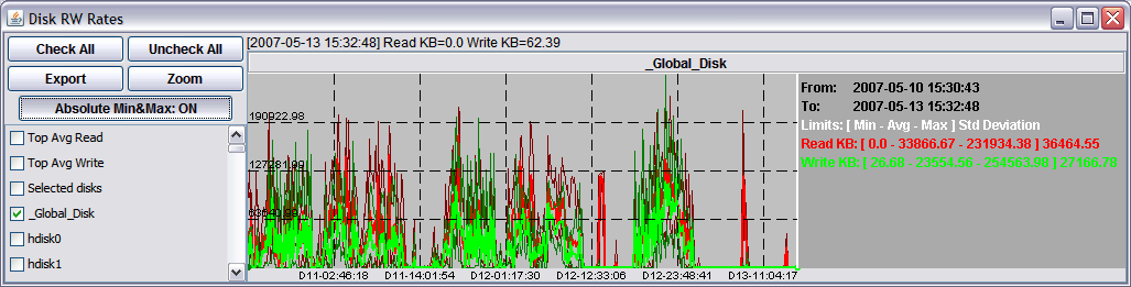
The Absolute Min&Max toggle button (on by default) changes graph content by showing a sort of error value around each graph. When dealing very big data files, many data samples should be displayed with the same x-axis position in the graph. pGraph averages all the values in the same x-axis position and shows only the average value. In order to provide a feeling of the distribution of values, pGraph also keeps track of absolute minimum and absolute maximum values on each x-axis position and shows such values with a darker and thinner line. The toggle button turns on and off the display of such values. In the previous figure the thinner lines are barely visible, providing a clue that in the selected time interval the average values represent a very good representation of the data.
When the mouse is moved on a graph, a vertical white bar appears and the status bar in the upper section of the window is updated. The status bar shows the time and the values related to the white bar in the graph pointed by the mouse. The bar is placed only on time point with valid data: if mouse moves on a point with no data, the bar is left on last valid point. If multiple data samples are related to the same x-axis position of the white line, the data is represented within square brackets providing the absolute minimum value, the average and the absolute maximum value in the x-axis position.
Each graph shows the current time window and the limits of each data set. Limits are always related to the time window and are updated at every zoom action. They show:
- The lower value in the time window (the absolute minimum)
- The average value in the time window
- The maximum value in the time window (the absolute maximum)
- The Standard Deviation value in the time window
Interactive graphs
Most graphs just show data related to the selected time window, but there are some graphs that change content depending on user selections.
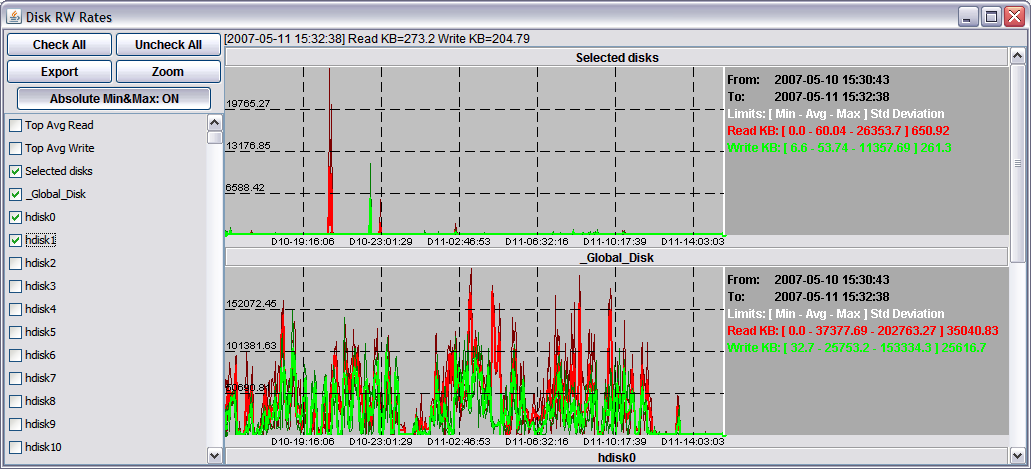
Selected items
In most windows there is one graph with a name that contain the "selected" word. This is a dynamic graph that sums data related to all selected graph in the same window and shows the result. If you change selection, the graph is automatically updated. This graph is very useful if you want to have information from a subset of data.
The following picture shows Read and Write data rates for disk. In the "Selected disk" panel only the sum of hdisk0 and hdisk1 data is shown, while the "_Global_Disk" panel contains data related the sum of all disk present in the system.
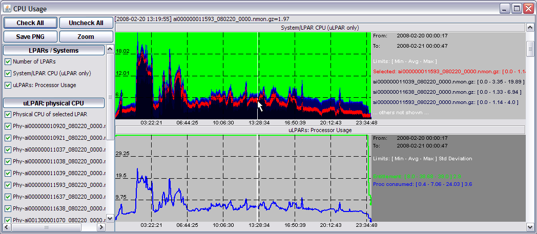
Stacked data
Some graphs show data as stacked areas to provide the idea of global resource usage and the components that use it. It is present in WLM window, Shared Processor Pool window and in CPU window when data is coming from multiple hosts. Each area is in blue with a different level of intensity, ordered by the average value on the metric (highest value on the bottom). On the right area there are labels related only to the top 3 or 4 contributors. If you move the mouse on the graph you can select a specific component that is pained in red and also shown on the label area.
In the following example there are two graphs related to CPU usage of a group of 10 LPARs. The "uLPAR: Processor Usage" shows the sum of all partition's processor usage. The "System/LPAR CPU (uLPAR only)" panel provides the same information but allows you to visually compare the contributors to CPU usage by moving the mouse and viewing data related to a specific LPAR.
Zoom Operation
All performance graphs are always related to the same time window to allow user to compare several metrics. By default the initial time windows it the one that contains all data extracted by all files read by pGraph. If user wants to change the time window, a Zoom operation must be performed.
When many data samples are near in time and must be shown on the same pixel of a graph, the value displayed is the average of all values that are related to the pixel. If a significant period of time is represented by a small number of pixels, some important information may be hidden and it may be useful to maze a zoom changing the display time window.
Zoom using main window
On the main window use the "Time Selection" section to select the time window to use. The central line represents the entire time period provided by performance data. The black ticks and labels and the grey area show the current time window used by graphs. You can use the two sliders to select a different time window: the red line and the red labels show the new proposed time. Once you have selected the new time window, press the Zoom button to update all graphs.
The following picture shows an example. All graphs are related to the time period from 2008-02-20 06:01:43 to 2008-02-20 16:50:05. A new time period has been selected from 2008-02-20 03:48:00 to 2008-02-20 19:39:33 but it has not been activated by pressing the Zoom button.
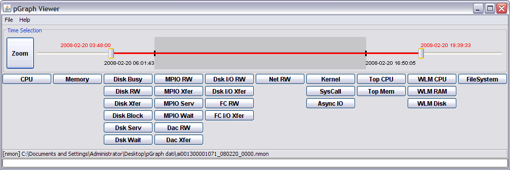
In the main window the upper section shows the current timeframe and provides button and sliders to change the time window. Any change in buttons and sliders will cause pGraph to read all files, select only data related to the new time window and update all graphs.
Zoom button
User can perform a Zoom on a narrower time window acting on any performance graph. The new time window is selected by clicking on the mouse button while moving the mouse pointer: two vertical bars on the graph will show the selected time window. A left click plus mouse movement selects the beginning of the time window, a right click plus mouse movement selects the end of the time window. The following picture shows an example:
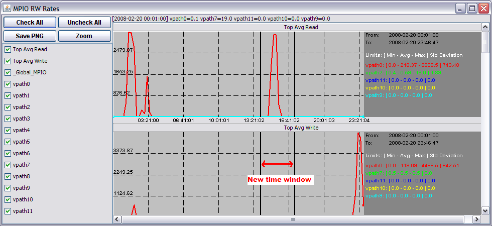
To activate the new time window, press the Zoom button. pGraph will read all data files and update all graphs in all windows.
Error management
By default each graph is 500 pixel width and all data samples in the selected timeframe are displayed in the graph. If the number of samples is smaller or equal to graph's width, the plotting is very simple: each sample is placed in its own pixel in the graph. When the number of samples is bigger, multiple data samples should be displayed in the same x-axis position in the graph and the result may become very confused. The more data is available in the selected time period, the more samples will share the same x-sample.
In order to simplify readability, pGraph averages all data samples that has the same x-axis position in the graph and keeps the absolute minimum and absolute maximum value for each position. The graph then shows a main line containing the average values and two darker and thinner lines that show the absolute minimum and absolute maximum values. The absolute min and max values can be turned on or off to have an idea of the error introduced by the averaging factor, as shown in the following figures:
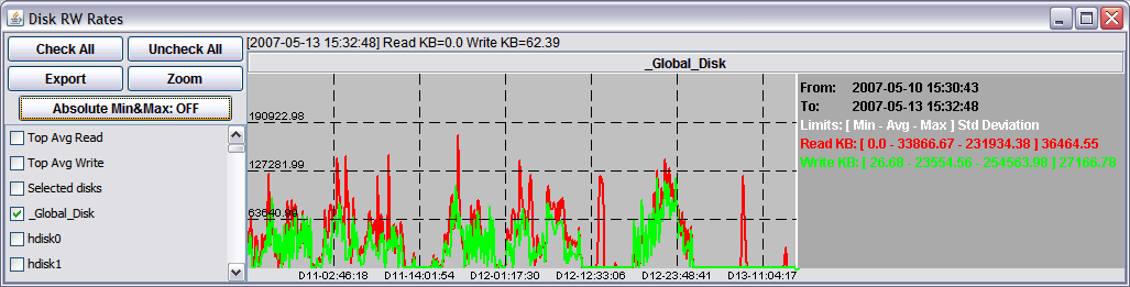
Absolute min and max values helps to to better understand the data. You may then choose to investigate further by performing a zoom on a smaller time period: the new graph will provide more clear details and a more defined graph.
Error management becomes extremely important when comparing data from multiple sources and providing a sum of values. Typical case is when you consolidate multiple LPARs on the same system and you want to evaluate global resource consumption (for example, CPU).
In order to keep memory usage low and constant regardless of the size of each data file, pGraph internally stores data in the same ways it displays it: average values for each x-axis place and absolute minimum and absolute maximum values. When pGraph computes the sum of multiple data sources, it is the average data that is added. Since computing errors are always additive, the result is a good representation but the error is increased. In order to keep error under control, pGraph updates the absolute min and max values of the resulting graph by adding the absolute minimum and absolute maximum of each graph. The final result is an average graph with a clear description of possible data variation.
The following examples shows how to manage the errors. Data has been collected from 6 LPARs and we are in charge of detecting the CPU load related to them. We have 6 nmon files, one for each LPAR, stored in the same directory and we use pGraph to load the directory (multiple hosts, multiple files). If we keep absolute min and max off, the following figure shows the global CPU consumption:
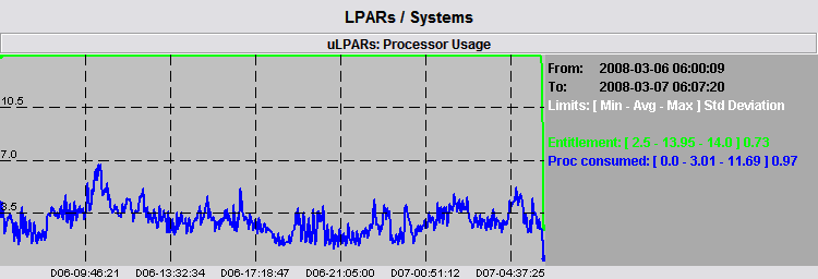
The graph shows that global average consumption a maximum value around 7.0 cores in the morning of day 06, while the legend tells us that there is an absolute maximum value of 11.69 somewhere. The absolute maximum represent the sum of absolute maximum of each of the 6 LPARs in a specific time slot. However, the time slot may include many data samples and the real sum may be lower than that. Only a time zoom around that time slot may provide accurate values.
In order to have a feeling of the range of real values, we can turn on the absolute minimum and maximum values and check the following figure:
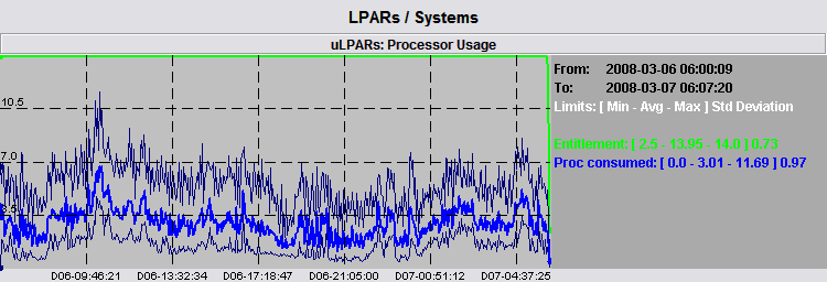
The real sum of CPU usage is in between the two light graphs. The average is a good representation of the sum of data but there are some peaks around it we may want to check. We immediately see that the biggest peak is really near the morning of day 06 and we can perform a zoom around such time, shown by the following picture.
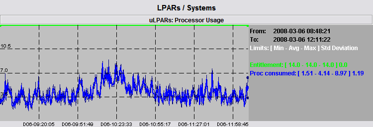
After performing the time zoom, the number of data samples to be considered is reduced and the graph shown becomes very accurate: there is a very little difference among average, absolute minimum and absolute maximum values. The absolute maximum has now a value of 8.97 and it is placed around 10.23 of day 06: this is the real maximum CPU usage of the 6 LPARs.
Error management becomes very important when the number of samples to be managed becomes very high (for example, when dealing with many days of data or a very short sampling time) of when the number of objects to be added is high (for example adding CPU usage of multiple LPARs or evaluating the I/O rate of many disks). Always check the absolute minimum and absolute maximum graphs to understand the possible variation of real data around the average graph.o
Additional Information
If you find errors or have question, email me:
- Subject: pGraph
- E-mail: vagnini@it.ibm.com
Document Location
Worldwide
| Version | Date posted | Package | Changes |
|---|---|---|---|
| 2.5.20 | 23 Sept 2024 | Several bug fixes | |
|
2.5.17 (current) |
10 June 2016 |
- Added 4KB and 64KB memory page statistics from NMON - Fixed CPI division by zero in lslparutil when LPAR is powered off |
|
| 2.5 | 12 April 2016 |
- Added page faults from NMON - Improved JFS change logging - CPI from lslparutil - Moved folded VPs on a dedicated panel - Stop reading disk data when new disks are added. - Skipping disk data when more than 100 disks. Use button to enable data parsing. - Added "Same max value" button in frames - Skipping JFS data when number of filesystems changes |
|
| 2.4 | 16 October 2012 |
|
Was this topic helpful?
Document Information
Modified date:
07 May 2025
UID
ibm11117185