Disclaimer - IBM Virtualization Best Practices Guide  

Copyright © 2025 by International Business Machines Corporation.

No part of this document may be reproduced or transmitted in any form without written permission from IBM Corporation. 

Product data has been reviewed for accuracy as of the date of initial publication. Product data is subject to change without notice. This information may include technical inaccuracies or typographical errors. IBM may make improvements and/or changes in the product(s) and/or programs(s) at any time without notice. References in this document to IBM products, programs, or services do not imply that IBM intends to make such products, programs or services available in all countries in which IBM operates or does business. 

THE INFORMATION PROVIDED IN THIS DOCUMENT IS DISTRIBUTED "AS IS" WITHOUT ANY WARRANTY, EITHER EXPRESS OR IMPLIED. IBM EXPRESSLY DISCLAIMS ANY WARRANTIES OF MERCHANTABILITY, FITNESS FOR A PARTICULAR PURPOSE OR NON-INFRINGEMENT. 

IBM shall have no responsibility to update this information. IBM products are warranted according to the terms and conditions of the agreements (e.g., IBM Customer Agreement, Statement of Limited Warranty, International Program License Agreement, etc.) under which they are provided. IBM is not responsible for the performance or interoperability of any non-IBM products discussed herein. 

The performance data contained herein was obtained in a controlled, isolated environment. Actual results that may be obtained in other operating environments may vary significantly. While IBM has reviewed each item for accuracy in a specific situation, there is no guarantee that the same or similar results will be obtained elsewhere. 

Statements regarding IBM’s future direction and intent are subject to change or withdrawal without notice and represent goals and objectives only. 

The provision of the information contained herein is not intended to, and does not, grant any right or license under any IBM patents or copyrights. Inquiries regarding patent or copyright licenses should be made, in writing to: 

IBM Director of Licensing     
IBM Corporation     
North Castle Drive Armonk, NY 10504-1785 U.S.A. 

Acknowledgments

We would like to thank the many people who made invaluable contributions to this document. Contributions included authoring, insights, ideas, reviews, critiques and reference documents. 

Our special thanks to key contributors from IBM Power Systems Performance: 

• Qunying Gao - Power Systems Performance

• Dirk Michel – Power Systems Performance

• Rick Peterson – Power Systems Performance

• Tom Tran – Power Systems Performance

Our special thanks to key contributors from IBM Development:

• Chris Francois – IBM i Development

• Pete Heyrman – PowerVM Development

• Stuart Jacobs – PowerVM Development

• Wade Ouren – PowerVM Development

• Dave Stanton – PowerVM Architecture & Development

• Dan Toft – IBM i Development

Our special thanks to key contributors from IBM i Global Support Center: 

• Kevin Chidester -IBM i Performance 

Our special thanks to key contributors from IBM Lab Services Power Systems Delivery Practice: 

• Eric Barsness –IBM i Performance 

• Tom Edgerton –IBM i Performance 

Preface

This document is intended to address IBM POWER processor virtualization best practices to attain best logical partition (LPAR) performance. This document by no means covers all the PowerVM^™ best practices so this guide should be used in conjunction with other PowerVM documents. 

Introduction    

This document covers best practices for virtualized environments running on POWER systems.   This document can be used to achieve optimized performance for workloads running in a virtualized shared processor logical partition (SPLPAR) environment.

Virtual processors

A virtual processor is a unit of virtual processor resource that is allocated to a partition or virtual machine.  PowerVM Hypervisor (PHYP) can map a whole physical processor core or can time slice a physical processor core. 

PHYP time slices shared processor partitions (also known as “micro-partitions”) on the physical CPU’s by dispatching and un-dispatching the various virtual processors for the partitions running in the shared pool.  The minimum processing capacity per processor is 1/20 of a physical processor core, with a further granularity of 1/100, and the PHYP uses a 10 millisecond (ms) time slicing dispatch window for scheduling all shared processor partitions' virtual processor queues to the PHYP physical processor core queues.
 

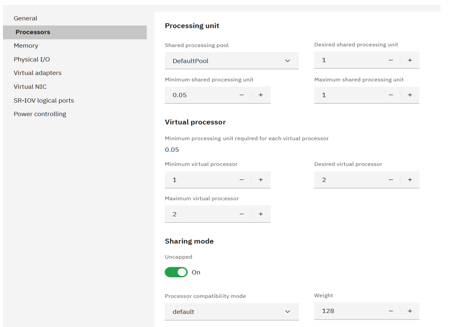
Figure 1. HMC processor configuration menu

If a partition has multiple virtual processors, they may or may not be scheduled to run simultaneously on the physical processors. 

Partition entitlement is the guaranteed resource available to a partition. A partition that is defined as capped, can only consume the processing units explicitly assigned as its entitled capacity.  An uncapped partition can consume more than its entitlement but is limited by several factors.    

Uncapped partitions can exceed their entitlement if there is unused capacity in the shared pool and there are dedicated partitions configured to share their physical processors while active or inactive 

• Unassigned physical processors are available
• COD utility processors have been configured    
   

If the partition is assigned to a shared processor pool, the capacity for all the partitions in the shared processor pool may be limited. The number of virtual processors in an uncapped partition throttles on how much CPU it can consume.  For example, an uncapped partition with 1 virtual processor can only consume 1 physical processor of compute capacity under any circumstances, and an uncapped partition with 4 virtual processors can only consume 4 physical processors of compute capacity.

Virtual processors can be added or removed from a partition using HMC actions. (Virtual processors can be added up to the Maximum virtual processors of an LPAR and virtual processors can be removed down to the Minimum virtual processors of an LPAR).    
 

Sizing/Configuring virtual processors 

The number of virtual processors in each LPAR in the system should not “exceed” the number of cores available in the system (CEC/framework) or if the partition is defined to run in specific shared processor pool, the number of virtual processors should not exceed the maximum defined for the specific shared processor pool. Having more virtual processors configured than can be running at a single point in time does not provide any additional performance benefit.  Instead context switching overhead of excessive virtual processors can reduce performance.   

For example:   A shared processor pool is configured with 32 physical cores. Eight SPLPARs are configured in this case each LPAR can have up to 32 virtual processors. This allows an LPAR that has 32 virtual processors to get 32 CPUs if all the other LPARs are not using their entitlement.   Setting > 32 virtual processors is not necessary as there are only 32 CPUs in the pool.  If there are sustained periods of time where there is sufficient demand for all the shared processing resources in the system or a shared processor pool, it is prudent to configure the number of virtual processors to match the capacity of the system or shared processor pool. 

A single virtual processor can consume a whole physical core under two conditions: 

• SPLPAR is given an entitlement of 1.0 or more processor 
• This is an uncapped partition and there is idle capacity in the system.    

Therefore, there is no need to configure more than one virtual processor to get one physical core. 

For example: A shared processor pool is configured with 16 physical cores.  Four SPLPARs are configured each with entitlement 4.0 cores. We need to consider the workload’s sustained peak demand capacity when configuring virtual processors. If two of the four SPLPARs would peak to use 16 cores (max available in the pool), then those two SPLPARs would need 16 virtual processors. The other two peak only up to 8 cores, those two would be configured with 8 virtual processors.    
 

Entitlement versus virtual processors 

Entitlement is the capacity that a SPLPAR is guaranteed to get as its share from the shared pool.   Uncapped mode allows a partition to receive excess cycles when there are free (unused) cycles in the system.   

Entitlement also determines the number of SPLPARs that can be configured for a shared processor pool.  That is, the sum of the entitlement of all the SPLPARs cannot exceed the number of physical cores configured in a shared pool. 

For example: Shared pool has 8 cores, 16 SPLPARs are created each with 0.1 core entitlement and 1 virtual processor.  We configure the partitions with 0.1 core entitlement since these partitions are not running that frequently.  In this example, the sum of the entitlement of all the 16 SPLPARs comes to 1.6 cores. The rest of the 6.4 cores and any unused cycles from the 1.6 entitlement can be dispatched as uncapped cycles.     

At the same time keeping entitlement low when there is capacity in the shared pool is not always a good practice.  Unless the partitions are frequently idle or there is a plan to add more partitions, the best practice is that the sum of the entitlement of all the SPLPARs configured should be close to the capacity in the shared pool.  Entitlement cycles are guaranteed, so while a partition is using its entitlement cycles, the partition is not preempted, whereas a partition can be preempted when it is dispatched to use excess cycles.  Following this practice allows the hypervisor to optimize the affinity of the partition’s memory and processors and it also reduces unnecessary preemptions of the virtual processors.    
 

Matching entitlement of an LPAR close to its average utilization for better performance 

The aggregate entitlement (min/desired processor) capacity of all LPARs in a system is a factor in the number of LPARs that can be allocated.  The minimum entitlement is what is needed to boot the LPARs, however the desired is what an LPAR will get if there are enough resources available in the system. The best practice for LPAR entitlement would be to match the entitlement capacity to average utilization and let the peak be addressed by additional uncapped capacity.   

 The rule of thumb would be setting entitlement close to average utilization for each of the LPARs in a system, however this rule can be relaxed when there are cases where a LPAR must be given higher priority compared to other LPARs in a system.  For example, if the production and non-production workloads are consolidated on the same system, production LPARs would be preferred to have higher priority over non-production LPARs. In which case, in addition to setting higher weights for uncapped capacity, the entitlement of the production LPARs can be raised while reducing the entitlement of non-production LPARs. This allows these important production LPARs to have better partition resource assignments (affinity) and these LPARs will have additional entitled capacity so not to rely solely on uncapped processing. At the same time if production SPLPAR is not using their entitled capacity, then that capacity can be used by nonproduction SPLPAR and the non-production SPLPAR will be pre-empted if production SPLPAR needs its capacity.        

When to add additional virtual processors     

When there is sustained need for a shared LPAR to use additional resources in the system in uncapped mode and there is available capacity, increasing virtual processors are recommended.   Keep in mind that this may negatively affect the performance of other partitions on the system if resources become constrained.     

How to estimate the number of virtual processors per uncapped shared LPAR     

The first step is to monitor the utilization of each partition and for any partition where the average utilization is ~100% one virtual processor can be added. That is, use the capacity of the already configured virtual processors before adding more. Additional virtual processors are going to run concurrently if there are enough free processors available in the shared pool.     

If the peak utilization is well below 50% mark, then there is no need for additional virtual processors.  In this case, look at the ratio of virtual processors to configured entitlement and if the ratio is > 1, then consider reducing the ratio.     

For AIX, if there are too many virtual processors configured, the operating system can “fold” those processors so that the workload would run on fewer virtual processors to optimize virtual processor performance.     

For example, if an SPLPAR is given a CPU entitlement of 2.0 cores and 4 virtual processors in an uncapped mode then the hypervisor could dispatch the virtual processors to 4 physical cores concurrently if there are free cores available in the system.  The SPLPARs leverages unused cores and the applications can scale up to 4 cores. However, if the system does not have free cores then the hypervisor would have to dispatch 4 virtual processors on 2 cores, so the concurrency is limited to 2 cores.  In this situation, each virtual processor is dispatched for reduced time slice as 2 cores are shared across 4 virtual processors. This situation could impact performance; therefore AIX operating system processor folding support may be able to reduce to number of virtual processors being dispatched such that only 2 or 3 virtual processors are dispatched across the 2 physical processors.   

IBM AIX virtual processor management – Processor folding

For AIX partitions, the operating system dynamically manages the number of active virtual processors through VPM (Virtual Processor Management), also known as processor folding. VPM folding will be enabled for dedicated processor partitions if static power saving has been enabled for the system. 

VPM determines the CPU utilization of the partition once per second and calculates the number of virtual processors needed based on the aggregate CPU usage plus an additional 20% for headroom. A virtual processor will be disabled (folded) if the aggregate CPU usage is below 80% of the enabled virtual processors. If available, an additional virtual processor will be enabled (unfolded) if the CPU usage is beyond 80% of the enabled virtual processors.     

VPM folding example    

The example below illustrates the unfolding of virtual processors. In this example the partition has eight virtual processors. The partition initially is idle and therefore has only one virtual processor unfolded.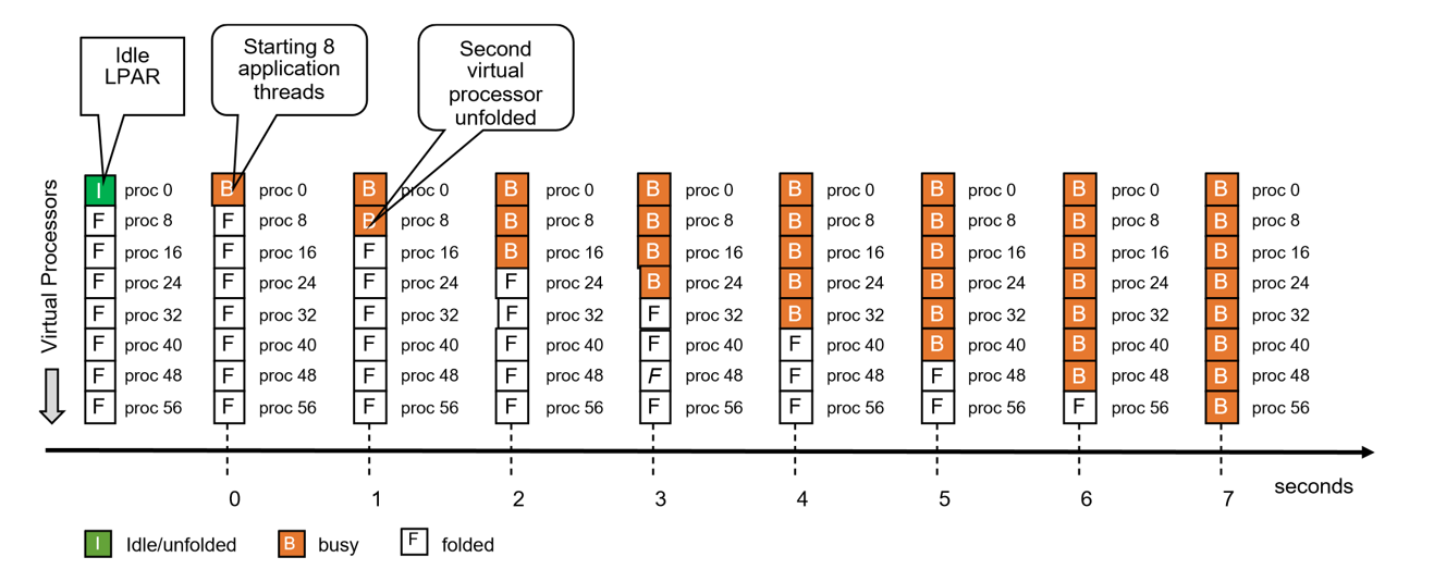


Figure 2. VPM folding example

• At 0 seconds we start a workload that consists of eight compute intensive application threads. At this time only one virtual processor is unfolded. Therefore, all application threads are running on one processor. In raw performance throughput mode, the application threads will mainly run on the primary SMT thread since overall partition utilization is too low to place them on the secondary or tertiary SMT threads. In scaled throughput mode the application threads will be placed on primary and secondary or on all SMT threads depending on which mode has been set.
• At 1 second an additional virtual processor gets unfolded since the aggregate CPU utilization of the enabled virtual processors exceeded the folding threshold. The same happens every second until all eight virtual processors are unfolded.

Note:The number of unfolded virtual processors will be lower when running scaled throughput mode since the eight application threads would be placed on four or two virtual processors.

Tuning virtual processor management folding 

For most workloads, unfolding one virtual processor per second is sufficient. However, some workloads are very response time sensitive and require available CPU resources immediately to achieve good performance. Disabling VPM folding would be one option but that would cause all virtual processors to be active all the time, whether they are needed or not. For most cases, a better way is to unfold more virtual processors in addition to the number determined by VPM. This can be done through the schedo tunable vpm_xvcpus. 

Taking the same example as in section 1.2.7 and setting vpm_xvcpus to 2 will unfold virtual processors as illustrated below:

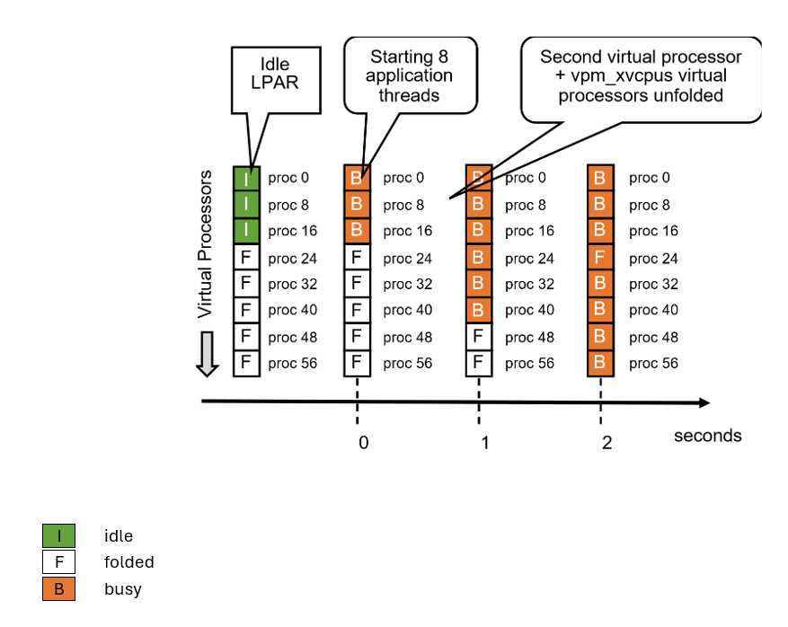
Figure 3. Virtual processor unfolding example

Like in the previous example, the partition has eight virtual processors. Three of the eight virtual processors are unfolded due to setting vpm_xvcpus=2. 

• At 0 seconds we start a workload that consists of eight compute intensive application threads. The eight application threads are now spread across the three unfolded processors.
• At 1 second VPM determined that one additional virtual processor is needed. Three were enabled before, so the new calculated value is four, plus the additional specified by vpm_xvcpus.
• At 2 seconds, all virtual processors are unfolded.

The example above uses a vpm_xvcpus value of 2 to demonstrate how quickly virtual processors are unfolded through vpm_xvcpus tuning. A vpm_xvcpus value of 1 usually is sufficient for response time sensitive workloads. 

Note: Tuning Virtual Processor Management folding too aggressively can have a negative impact on PHYP’s ability to maintain good virtual processor dispatch affinity. Please see section 3.4 which describes the relationship between VPM folding and PHYP dispatching. 

Power9/Power10/Power11 folding

VPM folding supports multiple SRADs (Scheduler Resource Allocation Domain) on Power9^™, Power10, Power11 shared processor partitions. VPM folds and unfolds virtual processors per SRAD. Virtual processors fold and unfold more quickly on shared processor partitions that have more than one SRAD. 

Relationship between VPM folding and PHYP dispatching 

VPM folding ensures that the number of active virtual processors is kept to what is really needed by the workload, plus a 20% additional headroom. This has a direct impact on PHYP’s ability to maintain good dispatching affinity in the case appropriate partition sizing was done based on the Virtualization Best Practices. 

The following example assumes a shared processor partition with 10 virtual processors and an entitlement of 6.0. The partition is placed in a shared processor pool that spawns across 24 cores and three 8-core chips. 

The figure below illustrates the shared processor pool with the placement of the home cores (entitled cores) within the pool. Please note that the partition placement of the illustration below represents a simplified example to explain the relationship between VPM folding and PHYP dispatching. Actual partition placement or placement rules are not covered in this section. 

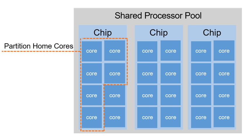
Figure 4. Partition home cores

Let’s assume that the workload put onto the partition consumes four physical core (PC 4.0) and that the shared processor pool is otherwise idle. With processor folding enabled, five virtual processors will be unfolded and PHYP can dispatch the virtual processor onto the home cores of the partition. 

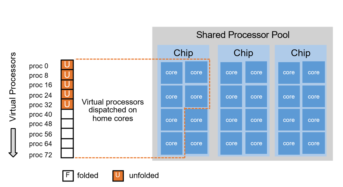
Figure 5. Shared partition placement with VPM folding enabled

The figure below illustrates what will happen running the same workload with VPM folding disabled. With VPM folding disabled, all 10 virtual processors of the partition are unfolded. It is not possible to pack all 10 virtual processors onto the five home cores if they are active concurrently. Therefore, some virtual processors get dispatched on other cores of the shared pool.

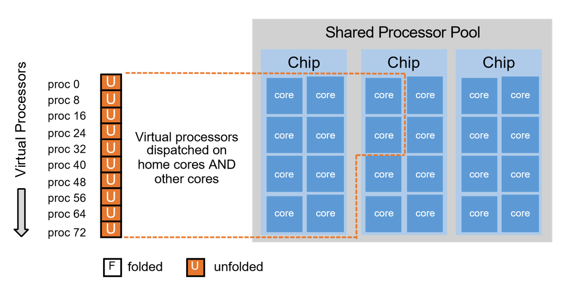
Figure 6. Shared pool core placement with VPM folding disabled

Ideally, the virtual processors that cannot be dispatched on their home cores get dispatched on a core of a chip that is in the same node. However, other chip(s) in the same node might be busy at the time, so a virtual processor gets dispatched in another node. 

For the example above, there is no performance benefit of disabling folding. More virtual processors than needed are unfolded; physical dispatch affinity suffers and typically the physical CPU consumption increases. 

AIX performance mode tuning 

AIX provides a dispatching feature through the schedo tuneable vpm_throughput_mode, which allows greater control over workload dispatching.  There are 5 options, 0,1,2,4 and 8 that can be set dynamically. Mode0 and 1 cause the AIX partition to run in raw throughput mode, and modes 2 through 8 switch the partition into scaled throughput mode. Starting with Power10, AIX default vpm_throughput_mode is set to 2 for shared processor partitions. For dedicated partitions, the default vpm_throughput_mode remains 0.

The default behavior is raw throughput mode, same as legacy versions of AIX.  In raw throughput mode (vpm_throughput_mode=0), the workload is spread across primary SMT threads. 

Enhanced raw throughput mode (vpm_throughput_mode=1), behaves similar to mode0 by utilizing primary SMT threads; however, it attempts to lower CPU consumption by slightly increasing the unfold threshold policy. It typically results in a minor reduction in CPU utilization.   

The new behavior choices are for scaled throughput mode SMT2 (vpm_throughput_mode=2), scaled throughput mode SMT4 (vpm_throughput_mode=4) and scaled throughput mode SMT8 (vpm_throughput_mode=8).  These options allow for the workload to be spread across 2 through 8 SMT threads, accordingly. The throughput modes determine the desired level of SMT exploitation on each virtual processor core before unfolding another core.  A higher value will result in fewer cores being unfolded for a given workload. 

Figure 7. Performance modes

AIX scheduler is optimized to provide best raw application throughput on Power9 – Power11 processor-based servers. Modifying the AIX dispatching behavior to run in scaled throughput mode will have a performance impact that varies based on the application.

There is a correlation between the aggressiveness of the scaled throughput mode and the potential impact on performance; a higher value increases the probability of lowering application throughput and increasing application response times.   

The scaled throughput modes, however, can have a positive impact on the overall system performance by allowing those partitions using the feature to utilize less CPU (unfolding fewer virtual processors). This reduces the overall demand on the shared processing pool in an over provisioned virtualized environment. 

The tunable is dynamic and does not require a reboot; this simplifies the ability to revert the setting if it does not result in the desired behavior.  It is recommended that any experimentation of the tunable be done on non-critical partitions such as development or test before deploying such changes to production environments.  For example, a critical database SPLPAR would benefit most from running in the default raw throughput mode, utilizing more cores even in a highly contended situation to achieve the best performance; however, the development and test SPLPARs can sacrifice by running in a scaled throughput mode, and thus utilizing fewer virtual processors by leveraging more SMT threads per core. However, when the LPAR utilization reaches maximum level, AIX dispatcher would use all the SMT8 threads of all the virtual processors irrespective of the mode settings.  

The example below illustrates the behavior within a raw throughput mode environment.  Notice how the application threads are dispatched on primary processor threads, and the secondary and tertiary processor threads are utilized only when the application thread count exceeds 8 and 16 accordingly. 

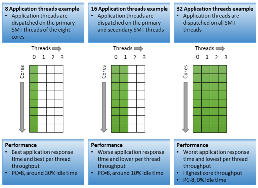
Figure 8. Application threads example

Processor bindings in shared LPAR 

Under AIX, binding processors is available to application running in a shared LPAR. An application process can be bound to a virtual processor in a shared LPAR. In a shared LPAR a virtual processor is dispatched by PowerVM hypervisor.  In firmware level 940 and later, the PowerVM hypervisor maintains three levels of affinity for dispatching, core, chip and node level. By maintaining affinity at hypervisor level as well as in AIX, applications may achieve higher level affinity through processor bindings. 

IBM i virtual processor management

Configuration of simultaneous multi-threading

The default SMT context for the LPAR’s virtual processors is selected by the Operating System, but it can be changed by the system administrator.  IBM i has historically selected the maximum supported SMT context as the default.  IBM i systems are typically operated with the default SMT context settings.

On POWER processors, SMT8 context offers maximum aggregate throughput and parallelism at full commitment, while allowing for increased single thread performance at lesser commitment/utilization levels.  Limiting the SMT context of the partition’s virtual processors can offer greater consistency in single thread performance, but with reduced aggregate throughput and capacity for parallelism.  In most IBM i environments, SMT8 context provides good single thread performance at typical utilizations and allows the system to absorb increases in workload that would otherwise overcommit the processor, leading to CPU queueing (i.e. dispatch latency) and its associated performance problems.

Processor multitasking mode

Selecting the SMT context for the partition virtual processors can be accomplished using the processor multitasking mode system value, QPRCMLTTSK.  Changes to the QPRCMLTTSK system value are effective immediately and persist across partition IPL.  The processor multitasking mode applies to all virtual processors of the partition.

Supported QPRCMLTTSK values are as follows:

• 0 - Processor multitasking is disabled. This value corresponds to single-thread (ST) context.
• 1 - Processor multitasking is enabled.  The SMT context is determined by the maximum SMT level control.
• 2 - Processor multitasking is system controlled. This is the default value, and the setting recommended by IBM. For Power8 and later processors, the implementation is identical to '1', with processor multitasking enabled.

Examples:

DSPSYSVAL SYSVAL(QPRCMLTTSK)            /* Display ST context */

CHGSYSVAL SYSVAL(QPRCMLTTSK) VALUE('0') /* Change to ST context */

CHGSYSVAL SYSVAL(QPRCMLTTSK) VALUE('1') /* Change to SMTn context */

CHGSYSVAL SYSVAL(QPRCMLTTSK) VALUE('2') /* Change to SMTn context */

Processor maximum SMT level

When processor multitasking is enabled, switching among available SMT contexts can be accomplished using the change processor multitasking information API, QWCCHGPR.  As with the QPRCMLTTSK system value, changes are effective immediately, persist across partition IPL, and are applicable to all virtual processors of the partition.

The QWCCHGPR API takes a single parameter, the maximum number of secondary threads per virtual processor:

0 – No maximum is selected.  The system uses the default number of secondary threads as determined by the operating system.

1-255 – The system may use up to the number of secondary threads specified.

Examples:

CALL PGM(QWCCHGPR) PARM(X'00000000') /* No maximum */    
CALL PGM(QWCCHGPR) PARM(X'00000001') /* SMT2 context */    
CALL PGM(QWCCHGPR) PARM(X'00000002') /* SMT2 context */    
CALL PGM(QWCCHGPR) PARM(X'00000003') /* SMT4 context */    
CALL PGM(QWCCHGPR) PARM(X'00000004') /* SMT4 context */    
CALL PGM(QWCCHGPR) PARM(X'00000007') /* SMT8 context */    
CALL PGM(QWCCHGPR) PARM(X'000000FF') /* SMT8 context */

Note that setting the maximum number of secondary threads does not establish the SMT context directly. The maximum value will be accepted regardless of the processor threading contexts supported by the underlying hardware, and the operating system will apply the configured maximum to the system.  If the QWCCHGPR API sets the maximum number of secondary threads to a value that is not supported by the hardware, the operating system sets the SMT context to the maximum supported by the hardware that satisfies the specified value.

The maximum number of secondary threads can be obtained from the retrieve processor multitasking information API (QWCRRTVPR). Note that the value returned is the maximum number of secondary threads configured.

Dispatch strategy

IBM i assigns workloads to the partition’s virtual processors to maximize throughput, while simultaneously avoiding entitlement delays and inefficient claims on unallocated (uncapped) processing capacity. The kernel’s dispatcher is responsible for the final placement of a ready-to-run process thread on a virtual processor thread, taking into account the thread’s long-term resource affinity domain assignment, workload capping group assignment, scheduling priority, and recent dispatch history.  In general, the dispatcher will spread workload across the number of virtual processors that are able to consume the partition’s entitled capacity.  For a partition that does not enjoy full entitlement (i.e. EC:VP = 1:1), the dispatcher spreads the workload across virtual processors up to the point where a claim on an additional virtual processor would consume capacity in excess of the entitled capacity.  At that point, the dispatcher attempts to pack additional workload into virtual processors already claimed.  Failing that, another virtual processor will be claimed, if available. Additional virtual processors in excess of the number that would exhaust entitlement are thus used sparingly.

The figure below depicts the dispatch of 8 application threads in various LPAR configurations, each having 8 virtual processors and entitled capacity 8.0, 4.0, 2.0, and 1.0 units respectively.

Processor folding

Processor folding increases the efficiency of the LPAR by managing the number of virtual processors available to the dispatcher.  The basic dispatch strategy tends to maximize the aggregate performance (and processing capacity consumption) of the available virtual processors.  The efficiency of the partition and/or system can be improved if the number of virtual processors available to the dispatcher is reduced to match the demand of the workload. Processor folding is a mechanism implemented by the Operating System to dynamically manage the number of virtual processors available for dispatching, based on LPAR configuration and placement, platform energy management settings, and workload characteristics.

Processor folding control system

The basic idea behind processor folding is for the Operating System to automatically manage the number of virtual processors available to the dispatcher for the purpose of improving efficiency, with the upper limit being the number of virtual processors active in the partition configuration.  For IBM i, the number of available virtual processors is primarily a function of the workload demand, parameterized by aspects of the LPAR configuration, SMT context, energy management policy, and other system settings. Workload demand is based on a statistical analysis of the number of dispatchable processor threads for each affinity resource domain, with the target number of virtual processors based on the mean and variance in the workload’s demand for processor threads. The number of available virtual processors increases and decreases with the demand for virtual processor threads. As depicted below, the processor folding control system is less restrictive when the number of virtual processors does not exceed the processor entitlement, and more restrictive when the number of virtual processors exceeds the entitlement.  Processor folding improves efficiency by confining the workload into fewer virtual processors than would otherwise be claimed.

Processor folding policy and configuration

In an IBM i partition, processor folding is configured and controlled by the Operating System by default.  On Power10 and earlier servers, the Operating System enables processor folding by default in shared processor LPARs or when Power Saving mode is enabled, or when Idle Power Saver is enabled and active in the platform.

On Power11 servers starting with IBM i 7.6, the Operating System also enables processor folding for dedicated processor LPARs configured for processor sharing, i.e. donating dedicated processors.  This policy change was phased-in to better align the capacity consumption characteristics of donating dedicated processor LPARs with those of fully entitled shared processor LPARs, without causing a behavior change for migration scenarios involving an Operating System or hardware change alone. Processor folding can be explicitly enabled in earlier releases and on earlier generations of POWER servers to similar effect, per examples below.

Operating System control of processor folding may be overridden via the QWCCTLSW limited availability API, which provides a key-based control language programming interface to a limited set of IBM i tunable parameters. Processor folding control is accessed via QWCCTLSW key 1060.  The following sequence of calls cycles through the various processor folding options. Changes to key 1060 take effect immediately but do not persist across partition IPLs. 

To get current processor folding status:

> CALL QWCCTLSW PARM('1060' '1')

KEY 1060 IS *SYSCTL.

KEY 1060 IS SUPPORTED ON THE CURRENT IPL.       

KEY 1060 IS CURRENTLY ENABLED.

To explicitly disable processor folding:

> CALL QWCCTLSW PARM('1060' '3')

KEY 1060 SET TO *OFF.

To explicitly enable processor folding:

> CALL QWCCTLSW PARM('1060' '2' 1)

KEY 1060 SET TO *ON. 

To re-establish Operating System control of processor folding policy:

> CALL QWCCTLSW PARM('1060' '2' 2)

KEY 1060 SET TO *SYSCTL.

LPAR page table size considerations

Each Logical Partition (LPAR) has a hardware page table which is used by the Power hardware to translate an effective address in partition memory to a physical real hardware address. The hardware page table of an LPAR is sized based on the maximum memory size of an LPAR and not what is currently assigned (desired) to the LPAR. For AIX, Linux and VIOS partitions, the default hardware page table ratio is 1:128 of the maximum memory for a partition.  For IBM i the page table by default is 1:64 of the maximum memory for a partition. For example, if the maximum memory is 128GB and this is an IBM i partition, 2GB would be set aside for the hardware page table.  You can change the default value for partition using the HMC.

Traditionally, Power has supported a single format of the data in the page table using a hashing algorithm.  The hashed page table is used for AIX, IBM i and VIOS partitions. Starting with Power10, Linux has switched from a hashed format to a radix tree format for compatibility with other server implementation of hardware page tables.  The radix tree format requires significantly less memory and based on experiments there is no performance loss in using a hardware page table ratio of 1:512 which is a savings of 4X over the default 1:128 page table size. Again, this only applies to Linux as only Linux supports radix page tables.

There are some performance considerations for hashed page tables (AIX, IBMi and VIOS) if the maximum size is set significantly higher than the desired memory. 

1. Larger page table tends to help performance of the workload as the hardware page table can hold more pages. This will reduce translation page faults. Therefore, if there is enough memory in the system and would like to improve translation page faults, set your max memory to a higher value than the LPAR desired memory.
2. On the downside, more memory is used for hardware page table; this not only wastes memory but also makes the table become sparse which results in a couple of things:
   1. Dense page table tends to help better cache affinity due to reloads.
   2. Lesser memory consumed by hypervisor for hardware page table more memory is made available to the applications.
   3. Page table walk time is better if the page tables are small.

Assignment of resources by the PowerVM Hypervisor

PowerVM resource assignment ordering 

When assigning resources to partition either at server boot or using the default options on the Dynamic Platform Optimizer, the hypervisor assigns resources one partition at a time until all partitions have been assigned resources. This implies that the partitions that are among the first to receive resources have a better chance of acquiring the optimum resources as compared to the last partitions to receive resources. The following is the order the hypervisor uses when determining the priority for resource assignment: 

1. Partitions that have explicit affinity hints like affinity groups
2. Partitions with dedicated processor partitions.
3. Higher uncapped weight for shared processor partitions.
4. Partition size (the more processors and memory a partition has, the higher the priority).

For example, all the dedicated processor partitions are assigned resource before any shared processor partitions.  Within the shared processor partitions, the ones with the highest uncapped weight setting will be assigned resources before the ones with the lower uncapped weights.    

Overview of PowerVM Hypervisor resource assignment    

 The hypervisor tries to optimize the assignment of resources for a partition based on the number of physical cores (dedicated processor partitions), entitled capacity (shared processor partitions), desired amount of memory and physical I/O devices assigned to the partition. The basic rules are:

• Try to contain the processors and memory to a single processor chip that has the most I/O assigned to the partition.
• If the partition cannot be contained to a single processor chip, try and assign the partition to a single DCM/Drawer that has the most I/O assigned to the partition.
• If the partition cannot be contained to a single DCM/Drawer, contain the partition to the least number of DCMs/Drawers.

Notes: 

• The amount of memory the hypervisor attempts to assign not only includes the user defined memory but also additional memory for the Hardware Page Table for the partition and other structures that are used by the hypervisor to manage the partition.
• The amount of memory available in a processor chip, DCM or Drawer is lower than the physical capacity. The hypervisor has data structures that are used to manage the system like I/O tables that reduce the memory available for partitions. These I/O structures are allocated in this way to optimize the affinity of I/O operation issued to devices attached to the processor chip.

How to determine if an LPAR is contained within a chip or drawer/Dual Chip Module (DCM) 

Each of the Operating Systems supported on PowerVM based servers provide a method of reporting physical processors and memory resources assigned to an individual partition.  This section will explain a couple common characteristics of the information reported followed by instructions by OS type that can be used to display the resource assignment information. 

The OS output for displaying resources assignments have the following common characteristics:

• The total amount of memory reported is likely less than the physical memory assigned to the partition because some of the memory is allocated very early in the AIX boot process and therefore not available for general usage.
• If the partition is configured with dedicated processors, there is a static 1-to-1 binding between logical processors and the physical processor hardware. A given logical processor will run on the same physical hardware each time the PowerVM hypervisor dispatches the virtual processor. There are exceptions like automatic processor recovery which would happen in the very rare case of a failure of a physical processor.
• For partitions configured with shared processors, the hypervisor maintains a “home” dispatching location for each virtual processor. This “home” is what the hypervisor has determined is the ideal hardware resource that should be used when dispatching the virtual processor. In most cases this would be a location where the memory for the partition also resides. Shared processors allow partitions to be overcommitted for better utilization of the hardware resources available on the server so the OS output may report more logical processors in each domain than physical possible. For example, if you have a server with 8 cores per processor chip, a partition with 8.0 desired entitlement, 10 VPs and memory, the hypervisor is likely to assign resources for the partition from a single chip. If you examine the OS output with respect to processors, you would see all the logical processors are contained to the same single domain as memory. Of course, since there are 10 VPs but only 8 cores per physical processor chip, not all 10 VPs could be running simultaneously on the “home” chip. Again, the hypervisor picked the same “home” location for all 10 VPs because whenever one of these VPs runs the hypervisor want to dispatch the partition as close to the memory as possible. If all the cores are already busy when the hypervisor attempts to dispatch a VP, the hypervisor will then attempt to dispatch the VP on the same DCM/drawer as the “home”.

Displaying resource assignments for AIX 

From an AIX LPAR, the lssrad command can be used to display the number of domains a LPAR is using.  The lssrad syntax is: 

lssrad -av 

If the cores and memory are located in multiple processor chips in a single drawer or DCM the output would look similar to: 

REF1 SRAD    MEM     CPU 

1. 0     31806.31  0-31 
2. 0    31553.75  32-63 

REF1 is the second level domain (Drawer or DCM).  SRAD refers to processor chips.  The lssrad command results for REF1 and SRAD are logical values and cannot be used to determine actual physical chip/drawer/DCM information.    

Note that CPUs refer to logical CPUs so if the partition is running in SMT8 mode, there are 8 logical CPUs for each virtual processor configured on the management console.   

Displaying resource assignments for Linux 

From a Linux partition the numactl command can be used to display the resource assignment. 

The numactl syntax is: numactl -H 

If the processors and some memories are allocated from one chip and there is memory without any processors on another chip, the output would look like the following: 

available: 2 nodes (0-1) node 0 cpus: 

node 0 size: 287744 MB node 0 free: 281418 MB 

node 1 cpus: 0 1 2 3 4 5 6 7 8 9 10 11 12 13 14 15 16 17 18 19 20 21 22 23 

node 1 size: 480256 MB

node 1 free: 476087 MB node distances: node   0   1   0:  10  40 

 1:  40  10 

A node from Linux corresponds to an individual processor chip so in this example the partition is using resources from 2 processor chips.  On the first chip is 287,744 MB of memory and on the second chip is 480,256 MB of memory and 24 logical processors.  Since this partition is running in SMT8 mode, this corresponds to 3 virtual processors with 8 hardware threads per virtual processor.  

Displaying resource assignments for IBM i 

IBM i has support in the Start SST (STRSST command) and the Dedicated Service Tools (DST) interface to display the resource assignment for a partition.  The following steps can be used to display this information: 

1. Use the DST function or the STRSST command to start the service tool function. 
2. Select the Start a service tool. 
3. Select the Display/Alter/Dump.
4. Select the Display/Alter storage or Dump to printer. 
5. Select Licensed Internal Code (LIC) data. 
6. Select Advanced analysis (Note—you may need to roll to see additional options). 
7. Enter 1 in the option column and enter rmnodeinfo in the command column. 
8. Enter -N in the Options prompt. 

The following is an example of the output from the rmnodeinfo command: 

 Running macro: RMNODEINFO -N  rmnodeinfo 

 macro start at 02/18/2020 15:22:16 

 Node statistics for 2 nodes across 2 node groups 

 Node #                       |                  0 |                   1 | 

 ============================================================================== 

 Hardware node ID             |                  1 |                   2 | 

 Node group ID                |                  0 |                   1 | 

 Hardware group ID            |                  0 |                   2 | 

 # of Logical procs           |                 16 |                  16 | 

 # of procs folded            |                  8 |                  16 | 

 # main store pages | 000748DB | 0007B8A8 | 

This is an example of a partition that is spread across 2 processor chips (Node # 0 and 1).  The # of Logical procs field indicates there are 16 logical processors on each of the two processor chips.  The # main store pages field reports in hexadecimal the number of 4K pages assigned to each of the two processor chips. 

Affinity scoring

PowerVM uses a scoring system (0-100 where 100 is best possible score) on a partition and server basis to indicate how well aligned the processor cores and memory are with respect to affinity (Non-Uniform Memory Access). If the processors, memory, hardware page table and such could fit in the largest chip on the server and the partition is actually assigned to a single chip, the partition affinity score would be 100.  If for some reason the partition resources are not coming from a single chip, the score is degraded base on how spread the resources are with respect to the ideal placement.  The same concepts hold true for partition that could fit into a single DCM/drawer, multiple DCMs/drawers and such.

Minimum affinity scoring

Starting with Power11, the HMC has support added two partition attributes that define the minimum score and the action to take when the current affinity score is less than the minimum affinity score. The minimum affinity score can be any value from 0-100. A minimum of 0 indicates that there is no required minimum for the partition (this is the default value).  The actions to take if the current affinity score is less than the minimum score are:

• None is the default setting and indicates no action is to be taken if the current affinity score is less than the specified minimum affinity score.
• Warn indicates that on partition activation, Live Partition Mobility (LPM) or Remote Restart to another server, the HMC will report that the operation was completed successfully but the current affinity score was below the minimum affinity score.
• Fail with not allow the activation/LPM/Remote Restart to complete successfully and a message will be displayed (assuming the activation was from the HMC). If this is an activation request, using the HMC optmem command to improve the partition affinity score may raise the current affinity score to the minimum affinity score or it may require changes to the partition being activated or changes to other partitions on the server to improve the current affinity score. If the activation was initiated by the hypervisor (for example, timed power on) and the minimum affinity score cannot be achieved, the partition activation fails with a system reference code. For LPM/Remote Restart, the scoring issue is on the target server which may require the HMC optmem command before LPM/Remote Restart, after LPM/Remote Restart or changes may be required to existing partitions on the target server to improve the current affinity score.

Optimizing resource allocation for affinity 

PowerVM when all the resources are free (an initial machine state or reboot of the CEC) will allocate memory and cores as optimally as possible.  At server boot time, PowerVM is aware of all the LPAR configurations so, assignment of processors and memory are irrespective of the order of activation of the LPARs.   

However, after the initial configuration, the setup may not stay static. There will be numerous operations that can change the resource assignments: 

• Reconfiguration of existing LPARs with updated profiles 
• Reactivating existing LPARs and replacing them with new LPARs 
• Adding and removing resources to LPAR dynamically (DLPAR operations)

Note: If the resource assignment of the partition is optimal, you should activate the partition from the management console using the “Current Configuration” option instead of activating with a partition profile.  This will ensure that the PowerVM hypervisor does not re-allocate the resources which could affect the resources currently assigned to the partition.     

If the current resource assignment is causing a performance issue, Dynamic Platform Optimizer is the most efficient method of improving the resource assignment. More information on the optimizer is available later in this section.     

If you wish to try to improve the resource assignment of a single partition and do not want to use the dynamic platform optimizer, power off the partition, use the chhwres command to remove all the processor and memory resources from the partition and then activate the partition with desired profile.  The improvement (if any) in the resource assignments will depend on a variety of factors such as which processors are free, which memory is free, what licensed resources are available, configuration of other partitions and so on.     

Fragmentation due to frequent movement of memory or processors between partitions can be avoided through proper planning ahead of time.  DLPAR actions can be done in a controlled way so that the performance impact of resource addition/deletion will be minimal. Planning for growth would help to alleviate the fragmentation caused by DLPAR operations. 

Optimizing resource assignment – Dynamic platform optimizer 

A feature is available called the Dynamic Platform Optimizer.  This optimizer automates the previously described manual steps to improve resource assignments.  The following functions are available on the HMC command line: 

lsmemopt –m <system_name> -o currscore will report the current affinity score for the server.  The score is a number in the range of 0-100 with 0 being poor affinity and 100 being perfect affinity.  Note that the affinity score is based on hardware characteristics and partition configurations so a score of 100 may not be achievable. 

lsmemopt –m <system_name> -r sys -o calcscore [-p partition_names | --id partition_ids] [-x partition-names | --xid partition-ids] will report the potential score that could be achieved by optimizing the system with the Dynamic Platform Optimizer.  Again, a calculated score of 100 may not be possible. The scoring is meant to provide a gauge to determine if running the optimizer is likely to provide improved performance.  For example, if the current score is 85 and the calculated score is 90, running the optimizer may not have a noticeable impact on overall systems performance. The amount of gain from doing an optimization is dependent on the applications running within the various partitions and the partition resource assignments.  If the p, --id, --x and/or –xid parameters are specified with calcscore, this will approximate the score on a partition basis that could be achieved if the optmem command was run with the same parameters. 

Also note that this is a system-wide score that reflects all the resources assigned to all the partitions.  The resource assignments of individual partitions contribute to the system wide score relative to the amount of resources assigned to the partition (large processor/memory partition contributes more to the system wide score than small partition).  Making any configuration change (even activating a partition that wasn’t assigned resources previously) can change the overall score. 

lsmemopt -m <system_name> -r lpar -o currscore | calcscore [-p partition_names | --id partition_ids] [-x partition-names | --xid partition-ids] will report the current or potential score on a partition basis.  The scoring is based on the same 0-100 scale as the system wide scoring.  If the -p, --id, --x and/or –xid parameters are specified with calcscore, this will approximate the score on a partition basis that could be achieved if the optmem command was run with the same parameters. 

lsmemopt –m <system_name> displays the status of the optimization as it progresses. 

optmem –m <system_name> -o start –t affinity will start the optimization for all partitions on the entire server.  The time the optimization takes is dependent upon: the current resource assignments, the overall amount of processor and memory that need to be moved, the amount of CPU cycles available to run this optimization and so on.  See additional parameters in the following paragraphs. 

optmem –m <system_name> -o stop will end an optimization before it has completed all the movement of processor and memory. This can result in affinity being poor for some partitions that were not completed. 

Additional parameters are available on these commands that are described in the help text on the HMC command line interface (CLI) commands.  One option on the optmem command is the exclude parameter (-x or –xid) which is a list of partition that should not be optimized (left as is with regards to memory and processors).  The include option (-p or –id) is not a list of partitions to optimizes as it may appear. Instead it is a list of partitions that are optimized first, followed by any unlisted partitions and ignoring any explicitly excluded partitions.  For example, if you have partition ids 1-5 and issue optmem –m myserver –o start –t affinity –xid 4 –id 2, the optimizer would first optimize partition 2, then from most important to least important partitions 1, 3 and 5.  Since partition 4 was excluded, its memory and processors remain intact. 

Some functions such as dynamic lpar and partition mobility cannot run concurrently with the optimizer.  If one of these functions is attempted, you will receive an error message on the management console indicating the request did not complete. 

Running the optimizer requires some unlicensed memory installed or available licensed memory. 

As more free memory (or unlicensed memory) is available, the optimization will be completed faster.  Also, the busier CPUs are on the system, the longer the optimization will take to complete as the background optimizer tries to minimize its effect on running LPARs. LPARs that are powered off can be optimized very quickly as the contents of their memory does not need to be maintained. The Dynamic Platform Optimizer will spend most of the time copying memory from the existing affinity domain to the new domain. When performing the optimization, the performance of the partition will be degraded and overall there will be a higher demand placed on the processors and memory bandwidth as data is being copied between domains.  Because of this, it might be good to schedule DPO to be run at periods of lower activity on the server. 

When the optimizer completes the optimization, the optimizer can notify the operating systems in the partitions that physical memory and processors configuration have been changed.  Partitions running on AIX 7.2, AIX 7.1 TL2 (or later), AIX 6.1 TL8 (or later), VIOS 2.2.2.0 (or later) and IBM I 7.3, 7.2 and 7.1 PTF with MF56058 have support for this notification.  For older operating system versions that do not support the notification, the dispatching, memory management and tools that display the affinity can be incorrect. Also, for these partitions, even though the partition has better resource assignments the performance may be adversely affected because the operating system is making decisions on stale information.  For these older versions, a reboot of the partition will refresh the affinity. Another option would be to use the exclude option on the optmem command to not change the affinity of partitions with older operating system levels.  Rebooting partitions is usually less disruptive than the alternative of rebooting the entire server. 

Live Partition Mobility (LPM) AND DPO considerations for Linux 

The base Linux operating system evolved from a non-virtualized environment where there was a single VM per server. Because of this initial design, there are currently some design assumptions that impact some of the features available on PowerVM with respect to affinity. When a partition migrates from one server to another or if DPO is executed, the underlying resources assigned to the partition can change. For example, the partition may have had processors and memory from 3 nodes and after LPM or DPO the processor and memory are only assigned to 2 nodes. Linux design assumptions do not allow the new topology information to be presented to Linux, so the partition runs with stale information with respect to the resources assigned to the partition.

The performance effect of this stale information could result is some cases sub-optimal performance since Linux is making decisions based on outdated information. There are many cases though where there will be little to no noticeable performance effects. The situation that should be fine would be if the partition is placed on the same or fewer nodes when performing an LPM or DPO operation. For example, if the hypervisor was able to contain the partition to a single processor chip or single drawer, the operation is performed and the resulting resource assignment is similar, there should be little to no performance change. If a partition was nicely contained to a single chip or drawer but due to the lack for free resources the resource assignment after LPM or DPO caused the partition to receive resources from other nodes, the performance could be affected.

The following are some suggestions to help understand information about the resource assignments and ways to mitigate the effects:

• Even though the Linux numactl -H output does not reflect the current resource assignment, the HMC lsmemopt command does reflect the current resource assignment. If the score is high (score of 100 is perfect), this indicates the partition has good assignment of resources and performance should not be affected because of the stale information. If the score is low, performance could be affected.
• When performing LPM, you may want to migrate the partitions with the most memory and processors or the most performance sensitive partitions before other partitions. If a server has lots of free resources, the PowerVM hypervisor can optimize the assignment of resources. As resources start becoming consumed, this tends to “fragment” the available resources which could lead to less than ideal resource assignments.
• When performing DPO, you may want to prioritize the placement order using the - -id or -x option. These options indicate to the PowerVM hypervisor that the listed partitions should receive resource assignments before other partitions.
• The more installed resources (processors and memory) the more likely the PowerVM hypervisor can optimize the resource assignments. The resources do not have to be licensed; they just need to be installed. The hypervisor can optimize even if the resources are “dark” resources.
• There may be a performance improvement even with less than ideal resources that could be obtained if Linux is able to work with accurate resource assignment information. A partition reboot after LPM or DPO would correct the stale resource assignment information allowing the operating system to optimize for the actual resource configuration.

Affinity groups 

The following HMC CLI command adds or removes a partition from an affinity group: 

chsyscfg -r prof -m <system_name> -i name=<profile_name> lpar_name=<partition_name>,affinity_group_id=<group_id> 

where group_id is a number between 1 and 255 (255 groups can be defined -affinity_group_id=none removes a partition from the group. 

Affinity groups can be used to override the default partition ordering when assigning resources at server boot or for DPO.  The technique would be to assign a resource group number to individual partitions. The higher the number the more important the partition and therefore the more likely the partition will have optimal resource assignment.  For example, the most important partition would be assigned to group 255, second most important to group 254 and so on. 

Lpar_placement

Lpar_placement = 2 

 The management console supports a profile attribute named lpar_placement that provides additional control over partition resource assignment.  The value of ‘2’ indicates that the partition memory and processors should be packed into the minimum number of domains.  In most cases this is the default behavior of the hypervisor, but certain configurations may spread across multiple chips/drawers.  For example, if the configuration is such that the memory would fit into a single chip/drawer/book but the processors don’t fit into a single chip/drawer/book, the default behavior of the hypervisor is to spread both the memory and the cores across multiple chip/drawer/book.  In the previous example, if lpar_placement=2 is specified in the partition profile, the memory would be contained in a single chip/drawer/book but the processors would be spread into multiple chips/drawers/books.  This configuration may provide better performance in a situation with shared processors where most of the time the full entitlement and virtual processors are not active.  In this case the hypervisor would dispatch the virtual processor in the single chip/drawer/book where the memory resides and only if the CPU exceeds what is available in the domain would the virtual processors need to span domains.  The lpar_placement=2 option is available on all server models and applies to both shared and dedicated processor partitions. For AMS partitions, the attribute will pack the processors but since the memory is supplied by the AMS pool, the lpar_placement attribute does not pack the AMS pool memory.  Packing should not be used indiscriminately; the hypervisor may not be able to satisfy all lpar_placement=2 requests.  Also, for some workloads, lpar_placement=2 can lead to degraded performance.     

Lpar_placement = 8    

Starting in FW1060.40 a specialized partition-based affinity scoring method was added for in-memory DB applications.  If this attribute is specified, the partition affinity scoring changes to use a new algorithm that computes the affinity score based on how evenly balanced the processors and memory are assigned across processor chips. For example, if the partition is assigned to 6 processor chips, and each chip has 5 cores and 100 LMBs assigned, the affinity score would be 100 as its perfectly balanced.  If the situation was that the partition was assigned to 6 processor chips and one chip had 1 core and one chip had 10 cores, the partition would be considered unbalanced and would result in a low affinity score.  An affinity score of 50 or above indicates that the difference between the chip with the smallest number of resources and the chip with the most resources is no more than 50% above the resources assigned to the smallest chip.  Any score below 50 may want to be considered as a poor affinity score for production usage by an in-memory database application.  Note that this attribute does not affect how the resources are assigned to the partition, it only affects how the affinity score is calculated.    

Lpar_placement considerations for failover/disaster recovery     

Many customers use a pair or cluster of systems for recovery purposes where in the case of failure of partition or server the work is offloaded to another server.  The placement of these partitions upon physical boundaries (drawers/books) is something to consider when optimizing the performance in preparation for a failover situation.     

The entitlement of the partitions needs to accurately reflect the CPU consumption under normal load (i.e. if the partition is consuming 4.5 processor units on average, partition should be configured with at least 5 VPs and 4.5 processor units and not 5 VPs with 0.5 processor units. Since the hypervisor uses the entitlement to determine how much CPU a partition will consume, the resource assignments of partitions will not be optimal if the entitlement is undersized. After ensuring the entitlement is correct, the next step is to place partitions into hardware domains with spare capacity such that when a failover occurs, there is unused capacity available in the domain.     

As an example, let’s assume two 2-drawer model with 16 cores per drawer.  On server ONE is Partition A1 which is configured for 16 virtual processors (VPs) and 8.0 cores and Partition B1 also is configured for 16 VPs and 8.0 cores. Server TWO is similar configuration with partitions A2 and B2.  Without any other directive, the hypervisor may place partitions A1 and B1 into the same drawer since the resources can be contained within a drawer.  When running normally (non-failover), each server is only licensed for 16 of the 32 installed cores.  In the event of a failure of a server, the transactions that were being processed by A1 will failover to A2, same for B1 failing over the B2.   Also, for failover, all cores in the server are activated such that the workload can be contained in a single server. What would be ideal for placement in the failover scenario would be that partition A2 is contained in a drawer with 16 CPUs and similarly B2 is contained in a different drawer.     

If all cores were licensed, one way to achieve this placement would be to configure A2 and B2 with 16.0 entitlement even though only 8.0 entitlement is required in the normal situation.  Since each drawer has 16 cores, the hypervisor would be forced to place these partitions on different drawers.  Another way to achieve the desired placement is though the configuration of memory.  For example, if each drawer has 256GB of memory, you could set each partition to 8.0 cores, 16 VPs and 230 GB.  In this situation when the hypervisor tries to place the partitions, the memory requirements of A2 and B2 force the hypervisor to place the partitions in separate drawers.  Allocation of memory beyond 50% of the capacity of the drawers would force this split.     

Some users may consider using the Dynamic Platform Optimizer after a failover as a placement strategy but there is a performance cost involved in running the optimizer.  The partitions, as the resources are moved between domains, run a bit slower and overall there is more CPU and memory bandwidth demand for the system.  If there is sufficient unused capacity in the system or the optimization can be delayed to a time when there is unused capacity, then the Dynamic Platform Optimizer may have a role to play in some failover scenarios.     

Server evacuation using partition mobility 

There may be situations where there is a need to move multiple partitions from one server to another server or multiple servers using partition mobility, for example in the case of hardware maintenance or firmware upgrade.  In such a scenario, the order in which the partitions are migrated will influence the resources assigned to the partitions on the target server.  One option to handle this situation is to run the dynamic platform optimizer after all partitions are migrated to the target server.   Another option would be to move the partitions in order from most important to least important.  Moving partitions in this order allow the hypervisor to first optimize the allocation of the CPU and memory resources to the most important partitions.   

PowerVM resource consumption for capacity planning considerations 

PowerVM hypervisor consumes a portion of memory resources in the system; during planning stage take that into consideration to lay out LPARs.  The amount of memory consumed by the hypervisor depends on factors such as the size of the hardware page tables for the partitions, the number of I/O adapters in the system, and memory mirroring.  The IBM system planning tool  (http://www.ibm.com/systems/support/tools/systemplanningtool/) should be used to estimate the amount of memory that will be reserved by the hypervisor.     

Licensing resources (COD)     

Power systems support capacity on-demand where customers can license capacity on-demand as the business needs for computing capacity grows.  In addition to future growth COD resources can be used to provide performance improvement.     

Licensing for COD memory is managed as an overall total of the memory consumed and there is no specific licensing of individual logical memory blocks (LMBs) or DIMMs.  If there is COD memory installed on the system, this can provide performance benefits because the hypervisor can use all the physical memory installed to improve partition resource assignments.  For example, on a two-drawer system, each drawer has 256GB of installed memory but only 400GB of licensed memory, a 240GB partition can be created on one drawer and a 120GB partition on the second drawer.  In this case, all 400GB is available and can be divided between the drawers in a manner that provides the best performance.     

Licensing for COD processor is managed on an individual core basis.  When there are fewer licensed cores than installed cores, the hypervisor identifies cores to unlicensed and puts these cores into a low power state to save energy. Note, when activating additional cores, the hypervisor may dynamically change which cores are licensed and unlicensed to improve partition resource assignment.     

The dynamic platform optimizer can be utilized when configuration changes are made as a result of licensing additional cores and memory to optimize the system performance. 

Resource Groups

Overview     

Power11 introduces Resource Groups which provide the ability to segment core resources for workload and performance purposes. When used properly, Resource Groups can deliver increased workload performance due to greater NUMA isolation and improved virtual processor dispatching.     

This section provides detailed information on Resource Groups, examples on how to use them and provides a link to the Resource Groups Advisor tool that helps to validate proper configuration.

Affinity / Dispatcher considerations 

Hardware layout

Resource groups provide a way of restricting the cores that are used by the PowerVM Hypervisor to dispatch logical partitions. The following is a pictorial view of single E1080 system node (enclosure that provides the connections and supporting electronics to connect the processor with the memory, internal disk, adapters, and the interconnects that are required for expansion) with 10 cores per processor chip:

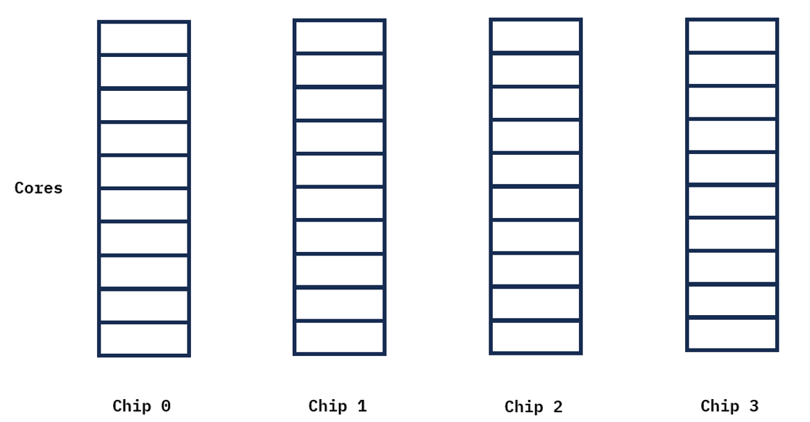
Figure 9. Cores across chips

The following is a pictorial view of resource groups where the system is divided into a resource group 1 with 8 cores, a resource group 2 with 2 cores and a resource group 3 with 30 cores.

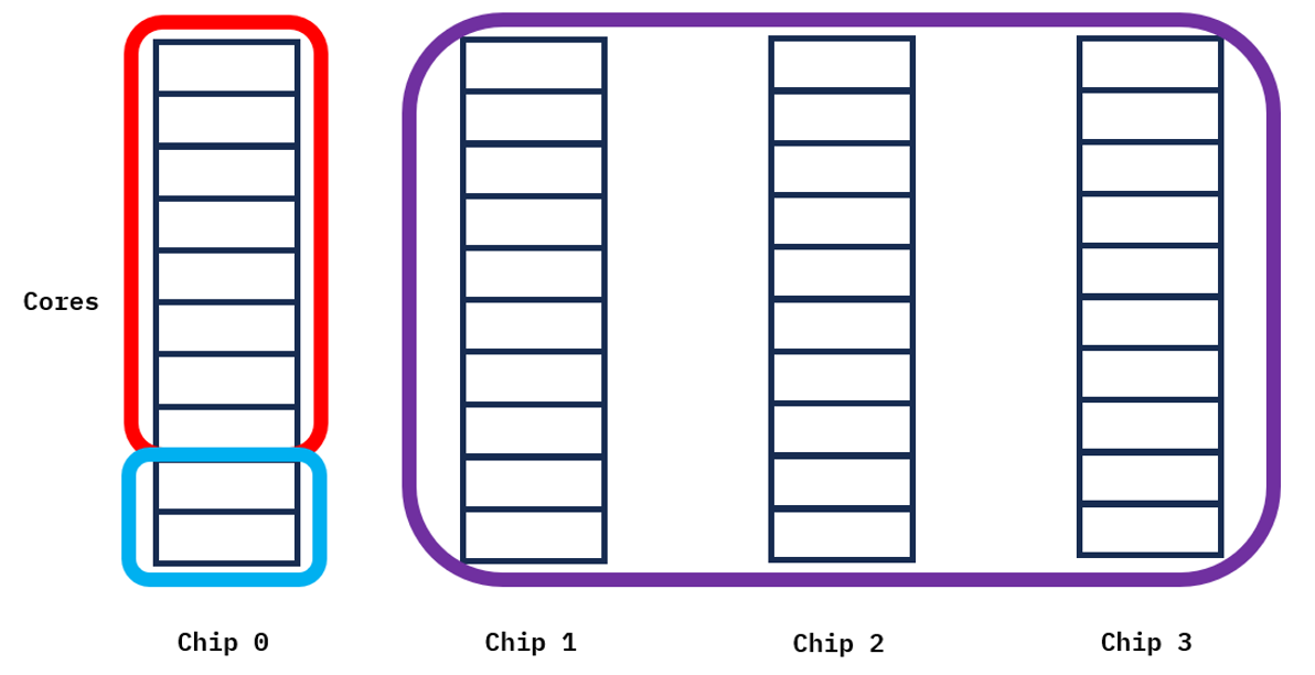
Figure 10. Resource groups across cores and chips

As the image shows, resource groups can be made up of any number of cores and can be spread across multiple processor chips, multiple DCMs or multiple system nodes.

Individual partitions (VIOS, AIX, IBM i or Linux) are assigned to an individual resource group.  One of the purposes of resource groups is to control the sharing of physical processor resources across a group of partitions.  Partitions will only be able to utilize cores assigned to the resource group and are not allowed to utilize cores from other resource groups. From figure 2, partitions assigned to resource group 1 will only be dispatched to run on the 8 cores selected from chip 0.  This is true for both dedicated and shared processor partitions.  Similarly with resource group 3 partitions could be dispatched on any of the 30 cores assigned to that group.  Restricting partition dispatches to a limited number of chips in some cases provides better and more consistent performance due to cache and non-uniform memory access (NUMA) times.

Virtual processor dispatching

Shared processor partition virtual processors (VPs) can be dispatched on cores that are configured as shared (either partition entitlement or shared processor pool reserve capacity), on cores that are not assigned to any partition and on cores that are assigned to dedicated partitions that allow sharing of the cores (either when the dedicated processor partition is inactive or active). Shared VPs cannot be dispatched on cores that are assigned to dedicated processor partitions that are configured to not share their processor resources or on any cores assigned to other resource groups.

For uncapped shared processor partitions, the determination of the next partition to be dispatched is made based on the uncapped weight of the partitions assigned to the specific resource group without impact from uncapped shared processor partitions in other resource groups.

Shared processor pools

Each resource group supports it own set of 64 shared processor pools (default shared processor pool and up to 63 user defined pools).  Shared processor pools provide a cap on the amount of CPU resources that can be consumed by the partitions assigned to the shared processor pool.  For example, if SharedPool01 is configured with a maximum of 5.0 processing units, the sum total of all partitions within a given resource group that are assigned to SharedPool01 cannot exceed 5.0 processor units. Limiting the CPU time for a group of partitions provides a mechanism to stay in compliance with software licenses. This capping can also be used to limit the CPU usage for a group of test partitions to allow for reserved capacity for production work within the same resource group.

Another consideration is that since each resource group has its own set of shared processor pools, software licenses need to be distributed across resource groups if applications using those software licenses are spread across resource groups.  For example, if you have 10 licenses from application X and multiple versions of this application are running in different resource groups, the max for the shared processor pools must be distributed across the resource groups running application X.

Memory considerations

When a partition is created, the PowerVM hypervisor tries to align the cores and memory allocated to the partition to provide the best performance.  For example, if the cores and memory can be contained on a single chip, that would provide the best performance.  In many situations it may not be possible to allocate all the cores and all the memory from the same set of processor chips.  A simple example would be if a 1 core partition is created but more than one chip’s worth of memory is assigned to the partition.  In this situation, there would need to be memory allocated from multiple chips but since there is only 1 core, that core is contained to a single chip.  It’s also possible that other partitions have consumed the best cores or best memory on chips such that some partitions have an uneven balance of memory and processors.

With resource groups, the possible set of cores that can be used for the partitions are limited to the cores owned by the resource group, but any installed licensed memory from any chip is available for partitions in any resource group.  This limiting of cores can provide more consistent and better performance but can also result in memory from outside the resource group being used to satisfy the memory requirements for the partition.  The PowerVM hypervisor always tries to allocate memory from the chips assigned to the partitions in the resource group but as described this might not always be possible.

If resource groups are defined on hardware boundaries (multiples of chips) and the partitions assigned to the resource groups are limited to the amount of memory associated with the cores assigned to the resource group, this will allow the PowerVM hypervisor to better align cores and memory.  For example, if a processor chip has 10 cores and 512GB of memory per chip and a resource group is created with 10 cores, then the total memory assigned to the partitions should be less than 512GB.  If the partitions require more than 512GB of memory and the performance is critical, then you may want to allocate 20 cores to the resource group so two chips are reserved.  If performance is not critical, it’s still a valid configuration to exceed 512GB of memory but the memory may be coming from other resource groups’ chips.  Partition size is not just the memory assigned to the partition but also includes structures to manage the partitions such as page tables, translation control entries for I/O operation and other virtualization structures.  The size of these structures can vary based on the individual partition configurations.

Creation of resource groups

Cores are assigned to a resource group at the time the resource group is created or updated.  The cores necessary to complete a request to create a resource group or increase the cores in an existing resource group must be available (not assigned to a resource group or partition).

From a performance perspective, when a resource group is created, the PowerVM hypervisor will attempt to assign cores with the best affinity, trying to contain the resource group to fewer chips whenever possible.  The following sections provide some insights into achieving the best possible resource assignment for resource groups.

New server

When creating resource groups on a new server, after the “all resources partition” is deleted, all of the cores are available and can be assigned to any resource group.  The first resource group that is created should be the one containing the most important partitions.  The second resource group the second most important partitions and so on.  This process ensures that the most important resource groups have the best possible assignment of cores.  The most important resource group should also be assigned the highest priority value so that at server power on or when Dynamic Platform Optimization (DPO) is run, it will be assigned the best possible cores.  Note, the default resource group always exists and has a default priority of 128.  As resource groups are created, the cores for the new resource groups are removed from the default resource group.

After the resource groups have been created, partitions can be created within the individual resource groups.

When resource groups are created, the PowerVM hypervisor does not have any information about the memory requirements of the partitions that will later be assigned to the resource groups.   As a result, it may be beneficial to reboot the server or use the HMC CLI optmem command to optimize the placement of the resource groups and partitions following their creation.

Existing server with Live Partition Mobility capabilities

If the system can use LPM, all partitions can be evacuated from a server prior to creating resource groups.  Once the resource groups are created, LPM can be used to return the partitions to the server.  When the partitions are moved to another server, this frees up all the cores on the server.  When partitions are returned to the original server, the resource group can be specified on the LPM request.  When using LPM, it is best to return the partitions in priority order, so the most important partitions have the best affinity assigned.  Once the partitions are restored, it may be beneficial to reboot the server or use the HMC CLI optmem command to optimize the placement of the resource groups and partitions.

Existing server without Live Partition Mobility capabilities

For existing servers that are not LPM capable, the following procedure can be used for initially setting up resource groups:

1. Power off all the partitions
2. Remove all the cores and memory from all the configured partitions using the HMC CLI chsyscfg command
3. Create the new resource groups
4. Assign the partitions to their resource groups
5. Activate the partition in priority order so the most important partitions receive the best possible resource assignment.

Once the partitions are activated, it might be beneficial to reboot the server or use the HMC CLI optmem command to optimize the placement of the resource groups and partitions.

Dynamic Platform Optimizer (HMC CLI optmem command) 

The HMC CLI optmem command has been enhanced to support optimizing the placement of partitions within a single resource group or optimize multiple resources groups and the placement of partitions in the non-excluded resource groups. More information about the resource group parameters (-g and --gid) can be found at https://www.ibm.com/docs/en/power11/9080-HEU?topic=commands-optmem.

Use case examples

There is a wide range of use cases where resource groups can be beneficial to performance by separating workloads. This section provides examples of how resource groups can be used to consolidate across multiple lines of business (client private cloud), isolate test and development from production, improve performance of multi-tiered workloads, system level isolation in multi-server consolidation, as well as improving performance by mapping shared processor pools into resource groups.

Consolidation across multiple lines of business

In this example, the Power10 server hosts the production, test and development partitions for two different departments, department "A" (green) and department "B" (blue). Each department has a database server, configured as a dedicated processor partition, and several shared processor partitions for test and development. Let's assume that CPU donation is enabled on the database partitions to donate unused CPU cycles to the shared processor pool.

Creating two resource groups, one for department "A" and one for department "B", allows for isolation of the partitions and workloads from the two departments.

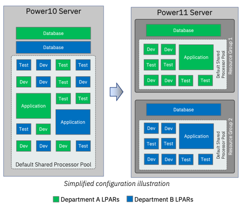
Figure 11. Resource group consolidation

Without resource groups:

• All shared CPUs are shared across the two departments.
• Donated CPU cycles can be used by any partition in the shared processor pool.

With resource groups:

• Each department can share the CPUs within their Resource Group.
• CPUs cannot be shared across Resource Groups. That is, department A cannot use the CPUs of department B's Resource Group or vice versa.
• Donated CPU cycles are only available to shared processor partitions within each resource group.

Isolation of production workloads from test/dev workloads

This example demonstrates how Resource Groups can be used to isolate production workloads from test and development workloads. The illustration below shows the Power10 server hosting a mix of application workload partitions along with test and development partitions. The CPUs from the default shared processor pool are shared across production, test and development workloads.

On Power11, creating a Resource Group for the test and development partitions allows for isolation of the production workloads from the test and development. The test and development partitions can only use the CPUs that are assigned to “Resource Group 1”. That is, there may be competition for CPU resources within “Resource Group 1” but such a competition will stay within “Resource Group 1”.

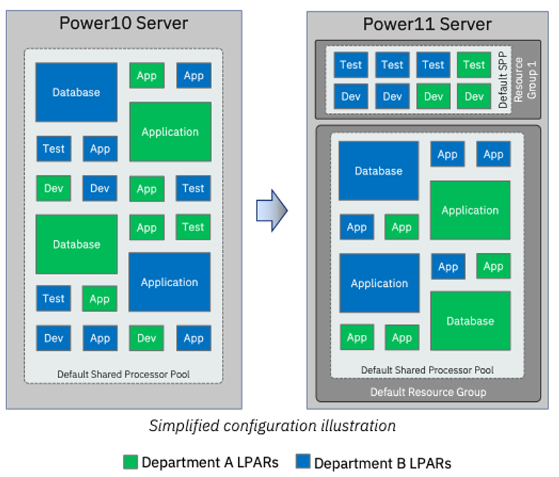
Figure 12. Resource group example

Improved application performance by grouping workload tiers into resource groups

Performance of multi-tiered workloads that communicate through virtual Ethernet benefit from close proximity. Ideally, partitions of a multi-tiered workload are placed on the same processor chip or socket (small partitions) or the same node on a multi-node server.

The illustration below highlights a multi-tiered workload, “Workload A” (partitions highlighted with a yellow border), that is hosted on a Power10 server. The partitions of this workload, a database and an application server, might be placed anywhere in the default shared processor pool. Let’s assume that they are placed on two different nodes of a multi-node server.

Creating a Resource Group for “Workload A” helps to improve the proximity of the database and application server partitions and therefore reduces latency in the communication over virtual Ethernet.

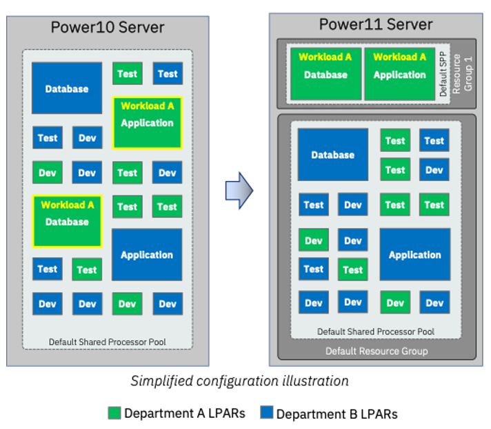
Figure 13. Simplified configurations with a resource group

System-level isolation in multi-server consolidation scenarios

The illustration below demonstrates how Resource Groups can be used to isolate workloads in a multi-server consolidation scenario.

On the left, the production, development and test workloads are physically isolated since each workload is running on its dedicated server.

Creating a Resource Group for each workload on Power11 provides a similar physical isolation like the dedicated servers.

Figure 14. Simplified configuration with resource groups

Combining use cases

Resource Groups are not limited to one of the previously described use cases. The use cases can be combined in multiple ways.

This example combines the consolidation across multiple lines of business together with isolating production from test and development by creating three Resource Groups:

• “Resource Group 1” for the production workload of department “A”.
• “Resource Group 2” for the production workload of department “B”.
• “Resource Group 3” for test and development for the two departments with the partitions of each department assigned to its own shared processor pool.

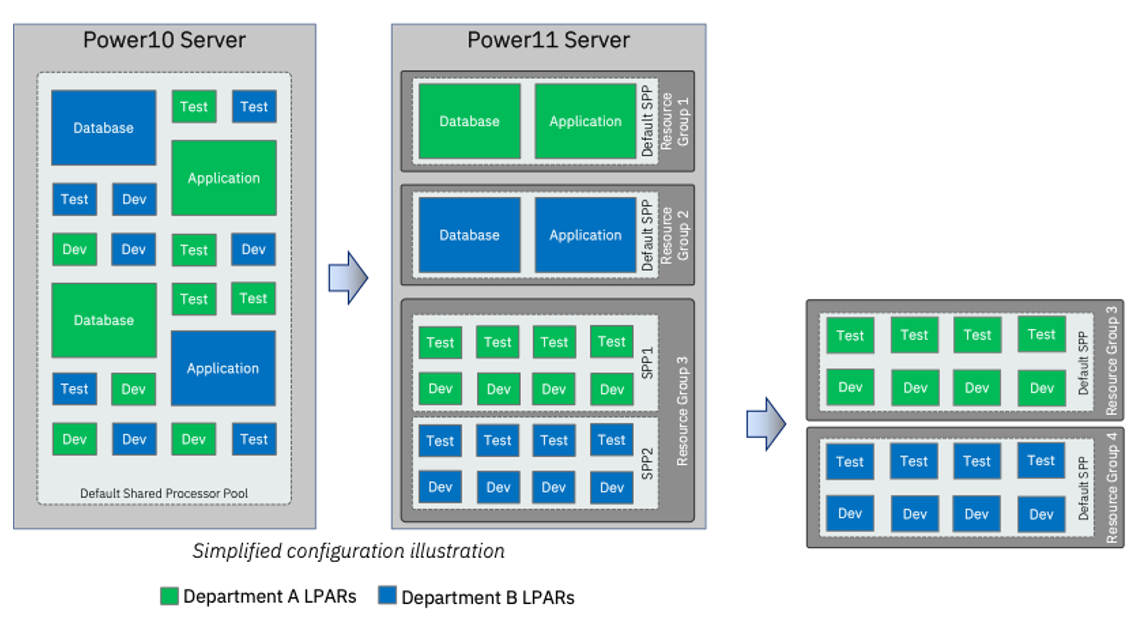
Figure 15. Resource group consolidation

More isolation between the test and development workloads of department “A” and “B” can be achieved by creating Resource Groups rather than shared processor pools.

Improving performance by mapping shared processor pools into resource groups

Resource Groups can help to improve performance of workloads that are running within a Shared Processor Pool.  This example shows multiple database partitions running in SPP1 (Shared Processor Pool 1) on a Power10 system.   In this scenario these database partitions are competing for and sharing physical cores with the application partitions in the default shared processor pool.

Creating a Resource Group with the same number of cores as SPP1 and moving the workload into a shared processor pool in this Resource Group isolates the database workload from all other workloads that are running on the system.  The database partitions in SPP1 inside of Resource Group 1 will not be competing for resources with or affected by the application partitions in the default resource group.

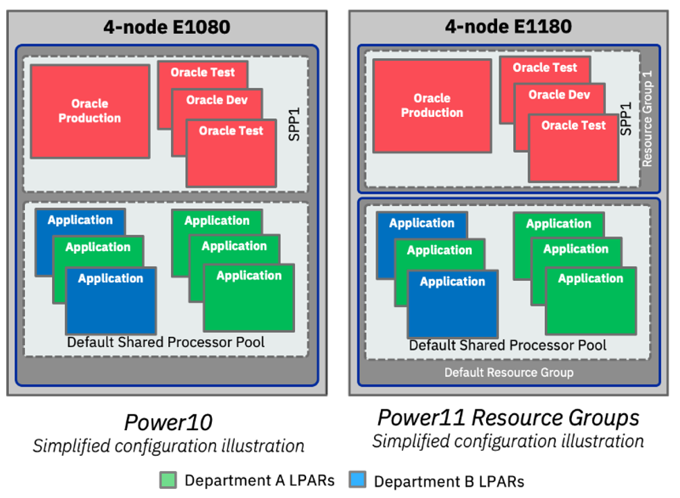
Figure 16. Isolating workloads using resource groups

Resource Groups Advisor

The benefits of resource groups will vary depending on the server configuration. Users migrating to a new Power11 server can use the Resource Groups Advisor (RGA) webtool to help evaluate if using resource groups is the right choice. RGA intakes the user's planned Power11 configuration including the proposed resource groups and outputs if using the proposed resource groups is recommended or not. RGA is available at https://www.ibm.com/it-infrastructure/resources/resource-groups-advisor.  
 

EnergyScale

IBM Power Systems utilize EnergyScale to optimize performance and energy consumption. EnergyScale allows systems to dynamically adjust processor frequency and power draw based on workload demands and environmental conditions.

There are three power management modes available: Max Performance mode, Static mode and Dynamic Performance mode. The setting of the mode can be done from HMC or ASMi, and it is dynamic so there is no need to reboot system or partitions. The power mode of partition is running can be checked by AIX command “lparstat -E 1 1”, if the mode is set to Dynamic or Maximum Performance mode, the reported mode can be changed based on the utilization. The processor frequency can be monitored by AIX command “lparstat -E “or Linux command of “ppc64_cpu –frequency”. For IBM i, the relative frequency can be displayed using WRKSYSACT. More details can be found at the following links:

• IBM EnergyScale for POWER9 Processor-Based Systems 
• IBM EnergyScale for POWER10 Processor-Based Systems      
• IBM EnergyScale for POWER11 Processor-Based Systems   

The three power management modes are: 

• Max Performance mode:Processor frequency will vary. This mode allows system to reach the maximum-frequency value.
• Static mode: Processor frequency will vary. This mode allows systems to reach mid-frequency value. Both max and statis mode allow system to reach to certain frequency by taking advantage of thermal and energy headroom provided by idle cores, lower workloads, and favorable environmental conditions.
• Dynamic Performance mode: The system firmware defaults to the maximum processor core frequency allowed for a system's environment and configuration. It also reduces frequency only when a system is less used or idle.

Processor compatibility mode

Processor compatibility modes provide IT software lifecycle benefits for IT infrastructure by ensuring the existing OS versions and application software you have deployed continue to run as intended. It is important to understand how processor compatibility modes impact your infrastructure when considering migrating to a new generation of Power, and the advantages of upgrading the OS version and application software to levels that support that latest generation of Power systems. New Instruction Set Architecture (ISA) features are only available in the mode that matches the current generation of the Power server you are deploying the workload on.

Each generation of Power systems supports compatibility modes from the previous two generations of Power systems, protecting your investment by allowing you to upgrade to a new generation without incurring downtime for a workload as part of the generational upgrade.

This table outlines the supported modes on each generation of Power systems:

Table 1 - Supported Processor Compatibility Modes

There is also a default setting available when deploying a partition on a Power system, which means the partition will run in the latest processor compatibility mode that the OS supports. This could potentially limit your LPM capability landscape. Best practice is that if you need flexibility with a mixed generation Power systems landscape to manage downtime and availability is to not use the default mode and specifically configure the mode based on your workload needs.

Additional information is available in the Power systems documentation:

• Power 9: Power 9: Processor Compatibility Mode definitions 

• Power10: Power 10 Processor Compatibility Mode definitions

• Power11: Power 11 Processor Compatibility Mode definitions

Conclusion

This document has described virtualization best practices for Power systems in order to configure your system and partition to help improve performance.   

Additional references are included in the next section. If you need additional help in assessing the potential impact of implementing LPARs, testing virtualization changes, or identifying ways to improve the performance of LPARs in your environment, please contact IBM Lab Services at ibmsls@us.ibm.com. 

References 

The following is a list of IBM documents that are good references: 

• IBM i on POWER – Performance FAQ https://www.ibm.com/downloads/cas/QWXA9XKN 
• Service and Support Best Practices https://www.ibm.com/support/pages/service-and-support-best-practices-power-systems
• IBM Power11 Redbook: https://www.redbooks.ibm.com/abstracts/sg248587.html
• Power Developer Portal Linux on Power  https://developer.ibm.com/search/?q=Linux%20on%20power
• System Planning Tool http://www.ibm.com/systems/support/tools/systemplanningtool/