Detailed reference: Edit Current Environment
The Edit Current Environment window presents a spreadsheet-like view within a browser window. In this view, you can view and edit the configuration and utilization profile, in addition, define scope.
Data that is loaded in this view is a snapshot of the current environment that is loaded by using Load config, or by adding servers, as described in Scenario: Adding more servers. You can then add to the data.
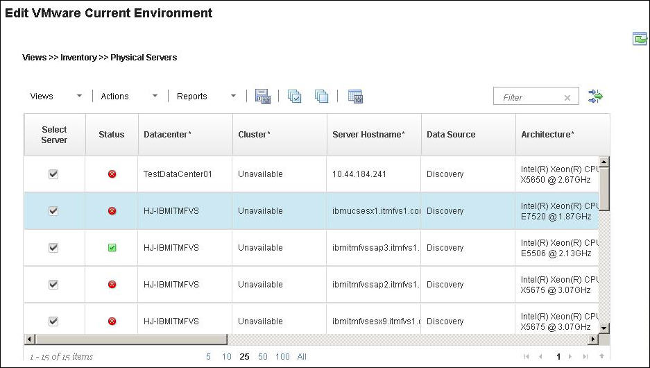
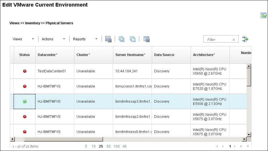
Physical server inventory view
- The Source tag ensures that during optimization, virtual machines from this physical server can only be moved to another physical server.
- The Target tag ensures that during optimization, this physical server can only receive virtual machines from another physical server.
- Source and Target tags together ensure that during optimization, virtual machines from the server can be moved for optimization and the server can also be used to place virtual machines.
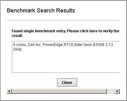
 icon indicates
that a single matching benchmark entry exists. A yellow triangle
icon indicates
that a single matching benchmark entry exists. A yellow triangle  icon
indicates that multiple benchmark matches to the server architecture
exist, but an approximate benchmark value is assigned to the server.
An X in a red circle
icon
indicates that multiple benchmark matches to the server architecture
exist, but an approximate benchmark value is assigned to the server.
An X in a red circle You can verify the search result by clicking the Status column. If multiple matches or no match, you can use the information from the search results to modify the architecture column to narrow down the match to the correct benchmark.
The built-in benchmark database of the Capacity Planner might not be complete with all the types and configuration variations (for example, vendor, model, architecture, number of cores, and so on) of physical servers that are available. Therefore, the Capacity Planner might not find an accurate benchmark value for the missing types and configuration variations.
In this case, you can feed in your environment-specific server data into the Capacity Planner database. This supplementary data is searched first before the built-in database by the Capacity Planner to find the benchmark values. For more information about the custom benchmark data, see the CUSTOM_USER_DEFINED_BENCHMARK.csv section in Editing knowledge base.
If the environment is homogeneous, use the raw CPU capacity option for analysis. Enable this option by updating the normalization benchmark setting as described inNormalization benchmark setting.
- Add Server
- You can add more physical servers to this view. These servers
can be used to provide additional hardware, or to try what-if scenarios.
When you choose this action, a window opens with a list of available
models, as shown in Figure 2.
You can select the appropriate model and create multiple instances
as needed.
When you click Create, a new row is added to the inventory grid with architecture details populated from the knowledge base data.
- Add Custom Tag
- You can extend and augment the discovered data with user-defined
attributes (tags). When you select this action, you are prompted to
provide the tag name and a new column is added to the inventory grid.
You can then add values for this column.
These tags can be used to formulate and apply rules during optimization. For more information, see Detailed reference: Edit Recommended Environment settings.
- Export Data
- You can download the data in the Physical Servers inventory view to a CSV file, which can be edited offline to add missing information.
- Import Data
- You can import a CSV file that was downloaded
using Export Data. Important: Note the following when you edit this file:
- The first column, Physical_Server_PK, must not be edited. If an extra physical server is added, you must keep the Physical_Server_PK column empty.
- Only previously NULL or blank data is updated. If data exists in a specified column, the data cannot be updated if edited.
Note: The Export and Import data supports the .zip file. The .CSV file is available in the .zip file.
Reports
The following reports are available:
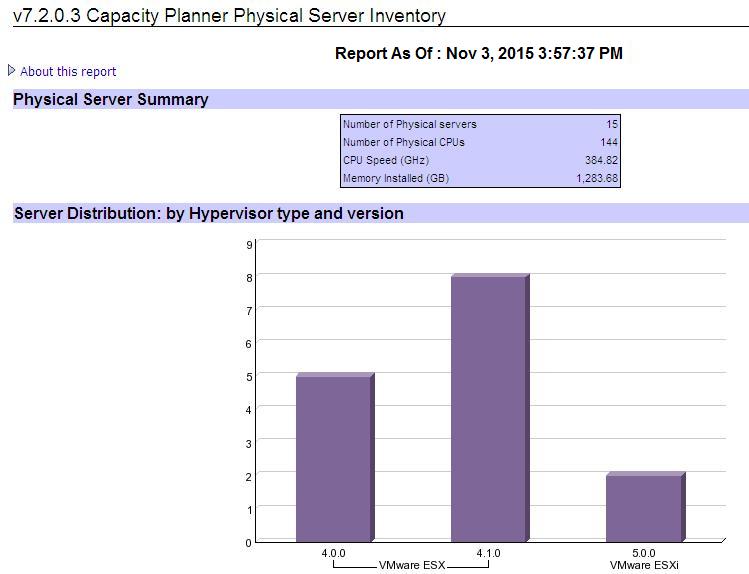
- Capacity Planner Physical Server Inventory
- The Capacity Planner Physical Server Inventory report presents
an overall view of the physical environment in the current Capacity
Planner session. The report contains a summary table of the inventory,
and bar charts that are organized by hypervisor name and version,
or data center and cluster, as shown in Figure 4.Figure 4. Capacity Planner Physical Server Inventory report
Virtual machine inventory view
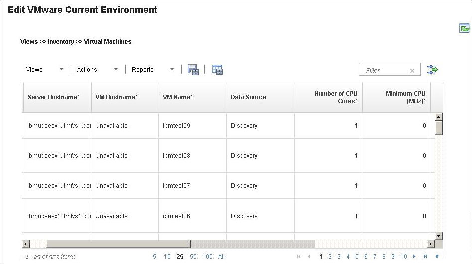
- Add Virtual Machine
- You can add a virtual machine to provide for future workloads. A new row is added to the inventory grid where you can populate details of the new virtual machine. Virtual Machines can be added to any server in the working set, if spare capacity exists for CPU and memory reservations.
- Add Custom Tag
- You can extend and augment the discovered data with user-defined
attributes (tags). When you select this action, you are prompted to
provide the tag name and a new column is added to the inventory grid.
You can then add values for this column.
These tags can be used to formulate and apply rules during optimization. For more information, see Detailed reference: Edit Recommended Environment settings.
- Export Data
- You can download the data in the Virtual Machines inventory view to a CSV file, which can be edited offline to add missing information.
- Import Data
- You can import a CSV file that was downloaded
by using Export Data. Important: Note the following when you edit this file:
- The first column, VIRTUAL_MACHINE_PK, must not be edited. If an extra virtual machine is added, you must keep the VIRTUAL_MACHINE_PK column empty.
- Only previously NULL or blank data is updated. If data exists in a specified column, it cannot be updated if edited.
Reports
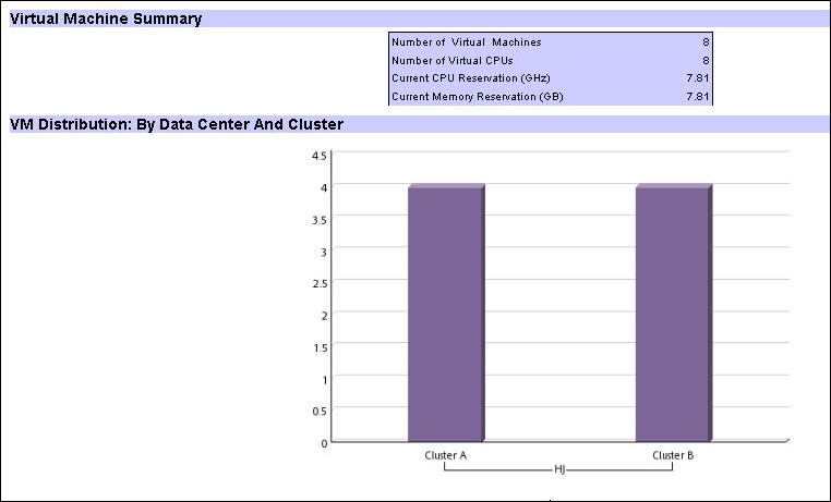
- Virtual Machine Inventory
- The Virtual Machine Inventory report presents an overall view
of the virtual environment in the current capacity planning session.
The report contains a summary table of the inventory and overall organizational
graphical representations that are organized by datacenter and cluster,
operating system name and version, and middleware name and version.
The report also contains bar charts that are organized by hypervisor
name and version, or data center and cluster, as shown in Figure 6.Figure 6. Virtual Machine Inventory report
Virtual Machines Utilization View
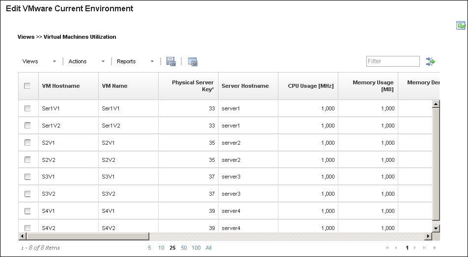
- Compute Usage
- You can compute the usage requirement of virtual machines by using
different parameters, as shown in Figure 8:Figure 8. Compute Usage windowCompute Usage calculates the sizing of the virtual machine for the parameters: CPU, memory, network bandwidth, and disk I/O usage. This sizing is done by analyzing the utilization data available in Tivoli Data Warehouse based on the summarization and aggregation levels specified. Aggregation levels available are Average, Minimum, Maximum, and 90th Percentile. Summarization levels available are Hourly, Daily, Weekly, Monthly, and Yearly. The available values in the Selected Summarization field depend on which value was selected in the Summarization field.
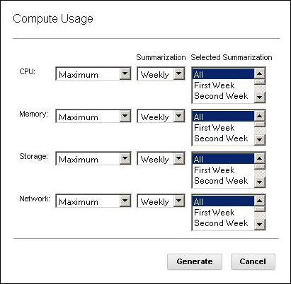 Important: Usage numbers are generated only for virtual machines that have utilization data that is collected in the Tivoli Data Warehouse.
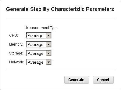
 - Generate Workload Stability Type
- The Generate Stability Characteristic Parameters window
is shown in Figure 9:Figure 9. Generate Stability Characteristic Parameters windowGenerate Workload Stability Type analyzes the hourly utilization data for a virtual machine and determines whether the resource utilization is stable or unstable, depending on the variation in usage.
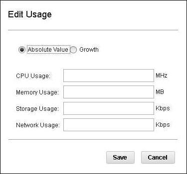
- Edit Usage
- The Edit Usage window is shown in Figure 10:Figure 10. Edit Usage windowYou can manually edit or Adjust-for-growth the resource usage. You can apply different growth profiles to adjust as needed. The usage parameters can be specified in absolute units, for example, 1024 MHz CPU, or a growth percentage can be applied, for example, add 10% growth to memory.
Reports
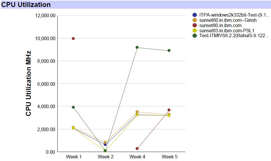
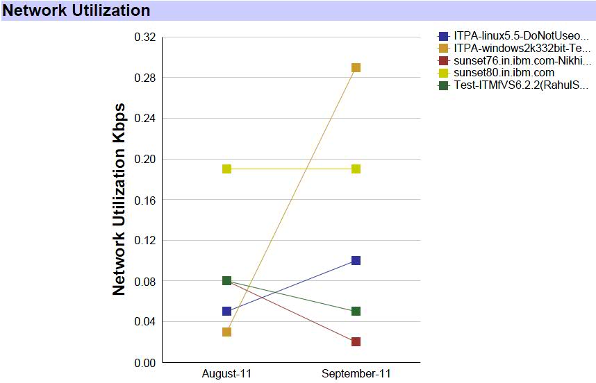
- Utilization Aggregated Timeseries report
- This report can be used to identify utilization patterns of virtual
machines. Because you can view aggregations of multiple virtual machines
at a time, you can also identify correlations in the resource utilizations.
You can use these observations to determine the usage sizing summarization
level. An example graph is shown in Figure 11.Figure 11. Utilization Aggregated Timeseries report
- Utilization Detailed Timeseries report
- This report helps you identify any data gaps in the utilization
data that is collected for the virtual machines Data points come directly
from aggregated measurement tables in utilization schema. An example
graph is shown in Figure 12.Figure 12. Capacity Planner Utilization Detailed Timeseries report
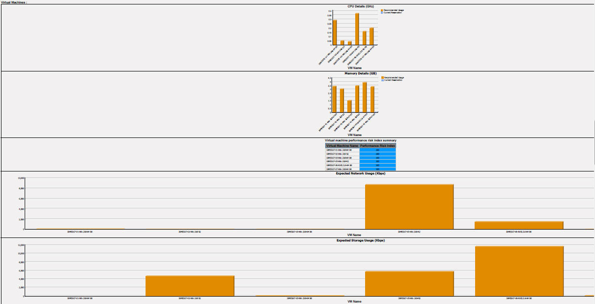
- Current Environment report
- The Capacity Planner Current Environment report shows the recommended
usage and sizing for each virtual machine that is based on time series
utilization data and sizing process: summarization, granularity type,
and selections. The report shows the capacity gaps, if any, in the
current environment before any optimization. Example output is shown
in Figure 13 and Figure 14.Figure 13. Current Environment report
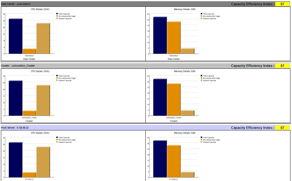 Figure 14. Current Environment report (continued)