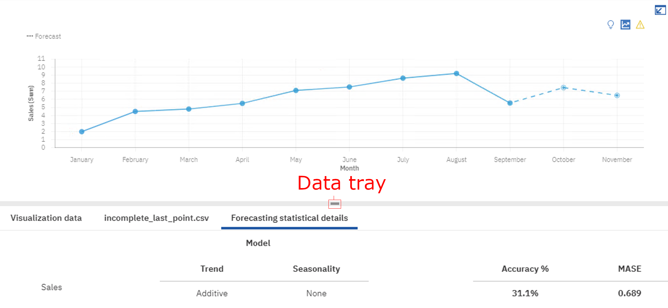
Forecasting statistical details

A forecasting run generates forecasts and forecasting statistical details. Forecasting statistical details are located in the data tray at the bottom of each visualization. There is a single row of statistical details for each time series in the visualization. Forecasting details are generated as long as the time points are evenly spaced.

Forecast information contains forecast Status for the given time series. When the status is Success, the other fields provide details on the model and data used for forecast. When the status is Failure, some of the other fields, including the Notes, provide details regarding the cause of the failure. Summaries of any failures are always provided in the visualization warnings.

Model information specifies the Trend and Seasonality type that is selected for estimating the time series data when successful. The following table lists the different available types.

Trend component	Seasonal component
	N NONE	A ADDITIVE	M MULTIPLICATIVE
N NONE	(N, N)	(N, A)	(N, M)
A ADDITIVE	(A, N)	(A, A)	(A, M)
Ad ADDITIVE_DAMPED	(Ad, N)	(Ad, A)	(Ad, M)

Trend component

Seasonal component

NONE

ADDITIVE

MULTIPLICATIVE

NONE

(N, N)

(N, A)

(N, M)

ADDITIVE

(A, N)

(A, A)

(A, M)

ADDITIVE_DAMPED

(Ad, N)

(Ad, A)

(Ad, M)

Accuracy measures

Model accuracy measures Mean Absolute Error (MAE), Mean Absolute Scaled Error (MASE), Accuracy Percent, Root Mean Squared Error (RMSE), Mean Absolute Percent Error (MAPE), and Akaike Information Criterion (AIC) are based on the time series data that is used to generate the model. All accuracy measures are based on the historical data. Accuracy measures can also be used as an indicator of the forecast accuracy, but they do not carry over to future values.

Mean Absolute Error (MAE): Computed as the average absolute difference between the values fitted by the model (one-step ahead in-sample forecast), and the observed historical data.
Mean Absolute Scaled Error (MASE): The error measure that is used for model accuracy. It is the MAE divided by the MAE of the naive model. The naive model is one that predicts the value at time point t as the previous historical value. Scaling by this error means that you can evaluate how good the model is compared to the naive model. If the MASE is greater than 1, then the model is worse than the naive model. The lower the MASE, the better the model is compared to the naive model.
Accuracy Percent (Accuracy %): The primary indicator of the model accuracy based on the fitted values. It is specified as the reduction percentage of mean absolute error relative to the naïve model. It is computed by subtracting MASE from 1 and expressing it as percentage. If MASE is greater than or equal to 1, the accuracy is set to 0% because the model does not improve upon the naïve model. Higher accuracy indicates lower model error relative to the naïve model.
Mean Squared Error (MSE): The sum of squared difference between the values that are fitted by the model, and observed values that are divided by the number of historical points, minus the number of parameters in the model. The number of parameters in the model is subtracted from the number of historical points to be consistent with an unbiased model variance estimate.
Root Mean Squared Error (RMSE): The square root of the MSE. It is on the same scale as the observed data values.
Mean Absolute Percent Error (MAPE): The average absolute percent difference between the values that are fitted by the model and the observed data values.
Akaike Information Criterion (AIC): A model selection measure. The AIC penalizes models with many parameters, and so attempts to choose the best model with a preference towards simpler models. The AIC is the sum of the logarithm of non-adjusted MSE multiplied by the number of historical points and the number of model parameters and initial smoothing states that are multiplied by 2.

Parameters

Detected Seasonal period and estimates for other parameters that are used in the selected exponential smoothing model are available.

Seasonal period: The number of time steps in a seasonal period used in the exponential smoothing model.
Alpha: The smoothing factor for level states in the exponential smoothing model. Small values of alpha increase the amount of smoothing, that is, more history is considered when the alpha is small. Large values of alpha reduce the amount of smoothing, which means that more weight is placed on the more recent observations. When the alpha is 1, all the weight is placed on the current observation.
Beta: The smoothing factor for trend states in the exponential smoothing model. This parameter behaves similar to alpha, but is for trend instead of level states.
Gamma: The smoothing factor for seasonality states in the exponential smoothing model. Serves the similar role as alpha, but for the seasonal component of the model.
Phi: The damping coefficient in the exponential smoothing model. Long forecasts can lead to unrealistic results, and it is useful to have a damping factor to dampen the trend over time and produce more conservative forecasts.

Diagnostics

Information includes Missing count, Series length, Ignored periods, Trend strength, Seasonality strength, and Date/time interval.

Missing count: Indicates the number of data rows that have either missing values or missing time points and are positioned between the first and the last valid series value. Invalid time points, as well as points with missing values at the first or the last historical time points are not included.
Series length: Indicates the number of data points used for time series modeling. Only the points between the first and the last valid series value are included.
Ignored periods: An integer, m, that ignores the last m data points of the series when building the exponential smoothing model and computing the forecasts. Any missing values at the end of a non-ignored portion of a series will also be forecast. The default value for this parameter is 0, which means that all of the historical data is used in model generation when there are no missing values. A maximum potential of 100 points can be ignored. Ignored periods excludes the data points when building a model, so forecasting might fail due to factors such as minimum data length requirements and missing value proportion that exceeds 33%.
Trend strength: Compare the original model, M, with the same model, but with the trend component removed. The trend strength of M is the difference in accuracy between model M and model M with the trend component removed.
Seasonality strength: Compare the original model, M, and the same model with the seasonal component removed. The seasonality strength of M is the difference in accuracy between model M and model M with the seasonal component removed.
Date / time interval: The Date / time interval represents the detected time interval of the chronologically sorted data. The time interval is identified as the smallest difference between neighboring points in the data when sorted in the chronological order.