Operator FFT
Specialized toolkits - release 4.3.1.0-prod20190605 > com.ibm.streams.timeseries 5.0.1 > com.ibm.streams.timeseries.analysis > FFT

The FFT operator applies a transformation of a time series from time domain into frequency domain. The FFT operator can be used for a number of different applications. For example, it can be used to decompose a time series signal into its constituent frequencies.
- Discrete Fourier Transform (DFT) with different variants
- inverse Discrete Fourier Transform
- Real Cepstrum transformation
- Discrete Cosine Transform (DCT)
- inverse Discrete Cosine Transform
Basics of the Discrete Fourier Transform
- The bandwith of the input signal is limited to the frequency f_c = 1/(2T), which is the critical or Nyquist frequency. This condition is required by the Sampling Theorem.
- Sampling of an input signal with the Dirac delta function results in a periodic spectrum with period 2 f_c, or 1/T.
- The discrete nature of the resulting spectrum, which can also be interpreted as sampling in the frequency domain, requires that the input signal is periodic, i.e. that the portion of analyzed data is continued periodically.
The following figure illustrates the periodic discrete spectrum, which is the result of a discrete Fourier Transform:
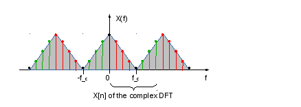
Formally, the DFT is the transformation of N complex numbers into N independent complex numbers. The result X[n] of the Discrete Fourier Transform contains terms at zero frequency, at positive, and at negative frequencies. You must remember that zero frequency corresponds to n = 0, positive frequencies 0 < f < f_c correspond to values 1 ≤ n ≤ N/2 −1, while negative frequencies −f_c < f < 0 correspond to N/2 +1 ≤ n ≤ N −1. The value n = N/2 corresponds to both f = f_c and f = −f_c. f_c is the critical or Nyquist frequency with f_c = 1/(2*T) or half the sampling frequency. The first harmonic X[1] corresponds to the frequency 1/(N*T).
There are many ways to define the DFT, varying in the sign of the exponent, normalization, etc. In this implementation, the DFT is mathematically defined as

while the discrete inverse Fourier Transform is defined as

It differs from the forward transformation in the sign of the exponent and the scaling factor 1/N.
For purely real input data, the spectrum has Hermitian symmetry, i.e. the negative frequency terms are just the complex conjugates of the corresponding positive-frequency terms, and the negative-frequency terms are therefore redundant. The size of the output for a real DFT is therefore only N/2 + 1, beginning with the frequency term at zero frequency and ending with the critical frequency at N/2. You can configure this type of Fourier Transform by using the algorithm parameter value realDFT, realFFT or its inverse inverseRealFFT.
The term N in the mathematical formulas is also referred to as the resolution of the transformation and has different constraints depending on the chosen algorithm. The resolution can be configured by using the resolution parameter or can be determined dynamically from the size of the input data or window size.
Basics of the Discrete Cosine Transform
The FFT operator can also be used to calculate the Discrete Cosine Transform of a signal. Mathematically, the discrete Cosine Transform transforms N real numbers x[0], ..., x[N-1] into N real numbers X[0], ..., X[N-1]. There are different variations regarding the assumptions about the continuation of the input signal and the scaling. The FFT operator can calculate the variant known as DCT II, which is defined as
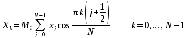
with the scaling factors

and for k > 0

These scale factors are the normalization used by Matlab, for example. The inverse DCT II is calculated as

where the X[j] are the scaled results from the forward transform.
Padding and Hamming-Windowing
- For complexFFT, inverseComplexFFT, realCepstrum, realFFT, and inverseRealFFT, the resolution must be a power of 2 and be at least 8.
- For realDFT, the resolution must be even and be at least 8.
- for DCT and IDCT, the resolution must be at least 8.
If the input size, i.e. the size of a list or a window, is smaller than the resolution requires, the data is padded at the end with zeros. Please note that padding with zeros should be strictly avoided if the input data of the operator represents a spectrum. Padding a spectrum at the end shifts the existing data points towards lower frequencies and turns negative frequency terms into positive ones if the input represents a two-sided spectrum.
Optionally a Hamming window can be applied to the input data before the transform happens. Please have in mind, that a window function, which is applied to a spectrum, effectively acts as a high pass if the input spectrum is two-sided or as a band pass if the input data represents a half-sided spectrum.
Operator input format
The FFT operator can ingest time series data in one of the following formats:
- float64
- list<float64>
- complex64
- list<complex64>
If the data being ingested is scalar (float64 or complex64), a window must configured. The amount of data (size of a list or window) for the transformation must be at least sufficient for a minimum resolution of 8, otherwise the portion of input data is dropped.
Operator outputs
The operator can produce three types of output:
- The result of the transform as a list<complex64>. For transformations with purely real results, like DCT and its inverse, real Cepstrum, and half-sided inverse Fourier Transform, the imaginary parts of the complex numbers are zero.
- The magnitude of the transform result as a list<float64>. These are the absolute values of the complex numbers.
- The square of the transformation result as a list<float64>. If the result is a spectrum, this can be interpreted is the power spectrum. It is calculated as the square of the absolute values from the complex output.
Behavior in a consistent region
- The FFT operator can be an operator within the reachability graph of a consistent region.
- The operator cannot be the start of a consistent region. An error occurs when you compile your streams processing application.
Summary
- Ports
- This operator has 1 input port and 1 output port.
- Windowing
- This operator optionally accepts a windowing configuration.
- Parameters
- This operator supports 5 parameters.
Required: algorithm, inputTimeSeries
Optional: flushOnFinal, resolution, useHamming
- Metrics
- This operator reports 1 metric.
Properties
- Implementation
- C++
- Threading
- Always - Operator always provides a single threaded execution context.
- Ports (0)
-
This port consumes the input time series to be transformed. The inputTimeSeries parameter specifies the name of the attribute on this port that contains the time series data. The accepted data types are float64, complex64, list<float64> and list<complex64>.
- Properties
-
- Optional: false
- ControlPort: false
- TupleMutationAllowed: true
- WindowingMode: OptionallyWindowed
- WindowPunctuationInputMode: WindowBound
- Assignments
- This operator allows any SPL expression of the correct type to be assigned to output attributes.
- Output Functions
-
- FFTCOF
-
- list<complex64> FFTAsComplex()
-
Returns the calculated FFT values.
- list<float64> magnitude()
-
Returns the absolute values of the complex results, for example a magnitude spectrum.
- list<float64> power()
-
Returns the square of the magnitude, for example a power spectrum.
- <any T> T AsIs(T v)
-
The default function for output attributes. By default, this function assigns the output attribute to the value of the input attribute with the same name.
- Ports (0)
-
This port submits a tuple that contains the transformed time series. This port submits a tuple each time a time series is transformed by the FFT operator. Custom output functions are used to specify the value of the output tuple attributes. The output tuple attributes whose assignments are not specified are assigned from input attributes.
- Properties
-
- Optional: false
- TupleMutationAllowed: true
- WindowPunctuationOutputMode: Generating
Required: algorithm, inputTimeSeries
Optional: flushOnFinal, resolution, useHamming
- algorithm
-
Specifies the type of spectral transform to perform. The supported algorithms are:
- complexFFT: Uses the complex Fast Fourier Transform algorithm that transforms N real or complex numbers into another N complex numbers. The complex FFT transforms a real or complex signal x[n] in the time domain into a complex two-sided spectrum X[n] in the frequency domain. You must remember that zero frequency corresponds to n = 0, positive frequencies 0 < f < f_c correspond to values 1 ≤ n ≤ N/2 −1, while negative frequencies −fc < f < 0 correspond to N/2 +1 ≤ n ≤ N −1. The value n = N/2 corresponds to both f = f_c and f = −f_c. f_c is the critical or Nyquist frequency with f_c = 1/(2*T) or half the sampling frequency. The first harmonic X[1] corresponds to the frequency 1/(N*T).
The complex FFT requires the list of values (resolution, or N) to be a power 2. If the input size if not a power of 2, then the input data will be padded with zeros to fit the size of the closest power of 2 upward.
The complex FFT is implemented as Cooley-Tukey algorithm, which has an effort of O(N * log (N)) in time.
-
inverseComplexFFT: Computes the inverse complex Fast Fourier Transform algorithm. The inverse complex FFT transforms a two-sided spectrum X[n], which is typically complex, into a complex signal x[n] in the time domain. This algorithm parameter value has the same conditions regarding the size of the input data as the complexFFT value.
The input data must be aligned as the output from complexFFT, first zero frequency, then positive frequencies, positive and negative Nyquist frequency at N/2, and finally the terms corresponding to the negative frequencies. Please note, that the input is a spectrum and the output is a signal in time domain. To get a real signal in time domain, the input must be complex and have Hermitian symmetry. For the inverse Fourier Transform, please ensure that the size of the input has the right value. It must be either the resolution value raised to the next power of two, or if resolution parameter is omitted, a power of two. Padding in frequency domain up to a size being a power of two will change the spectrum completely because the padded elements are added as zeros at negative frequencies, while the critical frequency is shifted. The critical frequency is always the element at N/2.
The inverse complex FFT is implemented as Cooley-Tukey algorithm, which has an effort of O(N * log (N)) in time.
-
realFFT: Uses the real Fast Fourier Transform algorithm. This value has conditions similar to the complexFFT value, except that the input data must be purely real. If the time series data has the basic type complex64, only the real parts of the complex numbers are used for the calculation. The imaginary parts are silently discarded.
The Fourier Transform of purely real input is Hermitian-symmetric, i.e. the negative frequency terms are just the complex conjugates of the corresponding positive-frequency terms, and the negative-frequency terms are therefore redundant. This parameter value does not compute the negative frequency terms, and the length of the complex output is therefore N/2 +1 . X[0] contains the zero-frequency term, which is real due to Hermitian symmetry. X[1] to X[N/2 -1] contain the terms at positive frequencies f > 0, while X[N/2] contains the term representing both positive and negative Nyquist frequency, which must also be purely real.
The real FFT is implemented as Cooley-Tukey algorithm, which has an effort of O(N * log (N)) in time. This algorithm is more efficient than complexFFT with subsequent ignoring the negative frequency terms.
-
inverseRealFFT: Performs the inverse real Fast Fourier Transform algorithm. A half-sided complex spectrum at the positive frequencies is transformed into a real time function. The complex return values of the FFTAsComplex() output function have zero imaginary parts, and the magnitude() returns the values of the real parts. This transformation assumes that the input spectrum has Hermitian symmetry (terms at negative frequencies are the complex conjugates of the terms at corresponding positive frequencies X(-f) = X*(f)). This special property requires that the terms at zero frequency and Nyquist frequency are real, while all others can have non-zero imaginary parts. To achieve this symmetry, the imaginary parts at these special points in the spectrum are silently discarded. The length of the input must be N/2 +1, with N being the resolution, which must be a power of 2. For the inverse Fourier Transform, please ensure that the size of the input has the right value. Padding in frequency domain will compress the spectrum shifting all existing frequency terms towards lower frequency. The last element of the input is always interpreted as the critical of Nyquist frequency.
The inverse real FFT is implemented as Cooley-Tukey algorithm, which has an effort of O(N * log (N)) in time. This algorithm is more efficient than inverseComplexFFT.
-
realDFT: Uses the real Discrete Fourier Transform (DFT) algorithm for purely real time functions. The conditions for the algorithm are the same as for realFFT, except that the length of the input data needs not be a power of 2. It can be any even number. If the length of the input is odd, a zero is padded to the input. The output is the one-sided complex spectrum at positive frequencies from X[0] to the critical or Nyquist frequency at X[N/2].
Notes:- This algorithm takes O(N * N) time, while the realFFT algorithm is of order O(N * log (N)) in time. For processing large signals, or when the length of the input is always a power of 2, the realFFT algorithm should be used.
- This algorithm has no inverse counterpart.
-
realCepstrum: Applies real Cepstrum transformation to a real input time series. The real Cepstrum is an N-to-N transformation of the following form:where
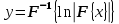 denotes the forward Fourier Transform and
 the inverse Fourier Transform.
In other words, the real Cepstrum of a real timeseries x is the inverse Fourier transform of the natural logarithm of the magnitude spectrum of x. The magnitude of the spectrum of a real time series is always an even real function. The logarithm does not change these properties. The inverse Fourier Transform of a purely real and even function is always a real function in the time domain.
The realCepstrum parameter value requires the size of the input data to be a power of 2. Otherwise padding will occur. The Cepstrum calculation involves two Fourier Transforms with effort of O(N * log (N)) in time.
-
DCT: Applies the Discrete Cosine Transform (DCT II) on the input time series. The DCT has no constraints regarding the resolution parameter value. As the DCT is a real-value transformation, the imaginary parts of complex input values are ignored, and the imaginary parts of the result are always zero.
The DCT is implemented as a matrix multiplication with O(N * N) effort in time.
-
IDCT: Applies inverse of the DCT II on the input time series. The inverse DCT has no constraints regarding the resolution parameter value. As the inverse DCT is a real-value transformation, the imaginary parts of complex input values are ignored, and the imaginary parts of the result are always zero.
The inverse DCT is implemented as a matrix multiplication with O(N * N) effort in time.
- Properties
-
- Type: FFT (realDFT, realFFT, inverseRealFFT, complexFFT, inverseComplexFFT, DCT, IDCT, realCepstrum)
- Cardinality: 1
- Optional: false
- ExpressionMode: CustomLiteral
- complexFFT: Uses the complex Fast Fourier Transform algorithm that transforms N real or complex numbers into another N complex numbers. The complex FFT transforms a real or complex signal x[n] in the time domain into a complex two-sided spectrum X[n] in the frequency domain. You must remember that zero frequency corresponds to n = 0, positive frequencies 0 < f < f_c correspond to values 1 ≤ n ≤ N/2 −1, while negative frequencies −fc < f < 0 correspond to N/2 +1 ≤ n ≤ N −1. The value n = N/2 corresponds to both f = f_c and f = −f_c. f_c is the critical or Nyquist frequency with f_c = 1/(2*T) or half the sampling frequency. The first harmonic X[1] corresponds to the frequency 1/(N*T).
- flushOnFinal
-
Specifies whether the pending tuples in the window are flushed when a final punctuation is received. If set to true, then the window is flushed and the window is processed. Be aware that data of a finally flushed window is most likely padded with zeros, which should be avoided if the input data represents a spectrum. If set to false, then the window is dropped and no processing occurs. The default value is false. If windowing is not enabled, this parameter is ignored.
- Properties
-
- Type: boolean
- Cardinality: 1
- Optional: true
- ExpressionMode: Constant
- inputTimeSeries
-
Specifies the name of the attribute that contains the time series data in the input tuple. The supported data types are float64, complex64, list<float64> and list<complex64>.
- Properties
-
- Type
- Cardinality: 1
- Optional: false
- ExpressionMode: Attribute
- resolution
-
Specifies the resolution value for the fast Fourier transform algorithm. The resolution is the N in the mathematical formulas. The supported algorithms (see the algorithm parameter) have different constraints regarding the resolution.
- For complexFFT, inverseComplexFFT, realCepstrum, realFFT, and inverseRealFFT, the resolution must be a power of 2 and at least 8.
- For realDFT, the resolution must be even and at least 8.
- for DCT and IDCT, the resolution must be at least 8.
If the resolution parameter is used, the parameter value is automatically raised to the next value that satisfies the constraints for the configured algorithm. If the resolution parameter is not used, the resolution is dynamically determined for each input list or each time the window triggers. In this case such a resolution value is chosen that the constraints of the algorithm are met, for example, if the input size is 12 and the algorithm is complexFFT, the resolution would be 16 because 16 is the next power of 2.
For the N-to-N and N-to-N/2+1 type transforms (all, except inverseRealFFT), the resolution parameter value cannot be less than the window size or the size of the time series list if now window is used. For the inverse half-sided FFT (inverseRealFFT), which is an N/2+1-to-N type transform, the resolution parameter cannot be less than 2 * (size -1), where size means the size of a configured window or the size of the time series list.
- Properties
-
- Type: uint32
- Cardinality: 1
- Optional: true
- ExpressionMode: AttributeFree
- useHamming
-
Specifies whether to use the Hamming window function before applying the transform algorithm. The default value is false. This parameter is useful only when the processed time series data represents data in the time domain. The Hamming window applied to a spectrum acts as a filter function in frequency domain.
- Properties
-
- Type: boolean
- Cardinality: 1
- Optional: true
- ExpressionMode: Constant
- FFT
-
stream<${schema}> ${outputStream} = FFT(${inputStream})
{
	param
		inputTimeSeries:		${timeSeriesExpression};
		algorithm:	${algorithmLiteral};

	output
		${outputStream}: ${outputExpression};
}
- numWindowsDropped - Counter
-
The number of times windows are dropped because they have less than the minimum time series values.
- No description for library.