ARIMA
With the ARIMA procedure you can create an autoregressive integrated moving-average (ARIMA) model that is suitable for finely tuned modeling of time series. ARIMA models provide more sophisticated methods for modeling trend and seasonal components than do exponential smoothing models, and they have the added benefit of being able to include predictor variables in the model.
Continuing the example of the catalog company that wants to develop a forecasting model, we have seen how the company has collected data on monthly sales of men's clothing along with several series that might be used to explain some of the variation in sales. Possible predictors include the number of catalogs mailed and the number of pages in the catalog, the number of phone lines open for ordering, the amount spent on print advertising, and the number of customer service representatives.
Are any of these predictors useful for forecasting? Is a model with predictors really better than one without? Using the ARIMA procedure, we can create a forecasting model with predictors, and see if there is a significant difference in predictive ability over the exponential smoothing model with no predictors.
With the ARIMA method, you can fine-tune the model by specifying orders of autoregression, differencing, and moving average, as well as seasonal counterparts to these components. Determining the best values for these components manually can be a time-consuming process involving a good deal of trial and error so, for this example, we'll let the Expert Modeler choose an ARIMA model for us.
We'll try to build a better model by treating some of the other variables in the dataset as predictor variables. The ones that seem most useful to include as predictors are the number of catalogs mailed (mail), the number of pages in the catalog (page), the number of phone lines open for ordering (phone), the amount spent on print advertising (print), and the number of customer service representatives (service).
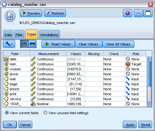
- Open the IBM® SPSS® Statistics File source node.
- On the Types tab, set the Role for mail, page, phone, print, and service to Input.
- Ensure that the role for men is set to Target and that all the remaining fields are set to None.
- Click OK.
- Open the Time Series node.
- On the Build Options tab, in the General pane, set Method to Expert Modeler.
- Select the ARIMA models only option and ensure that Expert
Modeler considers seasonal models is checked.
Figure 2. Choosing only ARIMA models 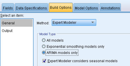
- Click Run to re-create the model nugget.
- Open the model nugget.
On the Output tab, in the left column, select the Model information. Notice how the Expert Modeler has chosen only two of the five specified predictors as being significant to the model.
Figure 3. Expert Modeler chooses two predictors 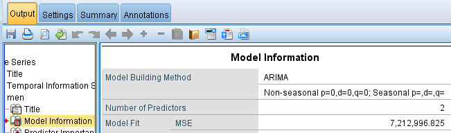
- Click OK to close the model nugget.
- Open the Time Plot node and click Run.
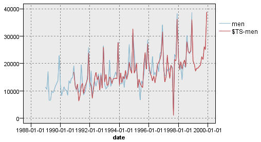
Figure 4. ARIMA model with predictors specified 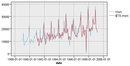
This model improves on the previous one by capturing the large downward spike as well, making it the best fit so far.
We could try refining the model even further, but any improvements from this point on are likely to be minimal. We've established that the ARIMA model with predictors is preferable, so let's use the model we have just built. For the purposes of this example, we'll forecast sales for the coming year.
- Click OK to close the time plot window.
- Open the Time Series node and select the Model Options tab.
- Select the Extend records into the future checkbox and set its value to 12.
- Select the Compute future values of inputs checkbox.
- Click Run to re-create the model nugget.
- Open the Time Plot node and click Run.
The forecast for 1999 looks good; as expected, there's a return to normal sales levels following the December peak, and a steady upward trend in the second half of the year, with sales in general above those for the previous year.